The first derivative test provides an analytical tool for finding local extrema, but the second derivative can also be used to locate extreme values. Using the second derivative can sometimes be a simpler method than using the first derivative.

We know that if a continuous function has a local extrema, it must occur at a critical point. However, a function need not have a local extrema at a critical point. Here we examine how the second derivative test can be used to determine whether a function has a local extremum at a critical point. Let [latex]f[/latex] be a twice-differentiable function such that [latex]f^{\prime}(a)=0[/latex] and [latex]f^{\prime \prime}[/latex] is continuous over an open interval [latex]I[/latex] containing [latex]a[/latex]. Suppose [latex]f^{\prime \prime}(a)<0[/latex]. Since [latex]f^{\prime \prime}[/latex] is continuous over [latex]I[/latex], [latex]f^{\prime \prime}(x)<0[/latex] for all [latex]x \in I[/latex] (Figure 9). Then, by Corollary 3, [latex]f^{\prime}[/latex] is a decreasing function over [latex]I[/latex]. Since [latex]f^{\prime}(a)=0[/latex], we conclude that for all [latex]x \in I, \, f^{\prime}(x)>0[/latex] if [latex]xa[/latex]. Therefore, by the first derivative test, [latex]f[/latex] has a local maximum at [latex]x=a[/latex]. On the other hand, suppose there exists a point [latex]b[/latex] such that [latex]f^{\prime}(b)=0[/latex] but [latex]f^{\prime \prime}(b)>0[/latex]. Since [latex]f^{\prime \prime}[/latex] is continuous over an open interval [latex]I[/latex] containing [latex]b[/latex], then [latex]f^{\prime \prime}(x)>0[/latex] for all [latex]x \in I[/latex] (Figure 9). Then, by Corollary [latex]3, \, f^{\prime}[/latex] is an increasing function over [latex]I[/latex]. Since [latex]f^{\prime}(b)=0[/latex], we conclude that for all [latex]x \in I[/latex], [latex]f^{\prime}(x)<0[/latex] if [latex]x0[/latex] if [latex]x>b[/latex]. Therefore, by the first derivative test, [latex]f[/latex] has a local minimum at [latex]x=b[/latex].

Figure 9. Consider a twice-differentiable function [latex]f[/latex] such that [latex]f^{\prime \prime}[/latex] is continuous. Since [latex]f^{\prime}(a)=0[/latex] and [latex]f^{\prime \prime}(a)<0[/latex], there is an interval [latex]I[/latex] containing [latex]a[/latex] such that for all [latex]x[/latex] in [latex]I[/latex], [latex]f[/latex] is increasing if [latex]x<a[/latex] and [latex]f[/latex] is decreasing if [latex]x>a[/latex]. As a result, [latex]f[/latex] has a local maximum at [latex]x=a[/latex]. Since [latex]f^{\prime}(b)=0[/latex] and [latex]f^{\prime \prime}(b)>0[/latex], there is an interval [latex]I[/latex] containing [latex]b[/latex] such that for all [latex]x[/latex] in [latex]I[/latex], [latex]f[/latex] is decreasing if [latex]x<b[/latex] and [latex]f[/latex] is increasing if [latex]x>b[/latex]. As a result, [latex]f[/latex] has a local minimum at [latex]x=b[/latex].

Note that for case iii. when [latex]f^{\prime \prime}(c)=0[/latex], then [latex]f[/latex] may have a local maximum, local minimum, or neither at [latex]c[/latex]. For example, the functions [latex]f(x)=x^3[/latex], [latex]f(x)=x^4[/latex], and [latex]f(x)=−x^4[/latex] all have critical points at [latex]x=0[/latex]. In each case, the second derivative is zero at [latex]x=0[/latex]. However, the function [latex]f(x)=x^4[/latex] has a local minimum at [latex]x=0[/latex] whereas the function [latex]f(x)=−x^4[/latex] has a local maximum at [latex]x=0[/latex] and the function [latex]f(x)=x^3[/latex] does not have a local extremum at [latex]x=0[/latex].

Let’s now look at how to use the second derivative test to determine whether [latex]f[/latex] has a local maximum or local minimum at a critical point [latex]c[/latex] where [latex]f^{\prime}(c)=0[/latex].

Example: Using the Second Derivative Test

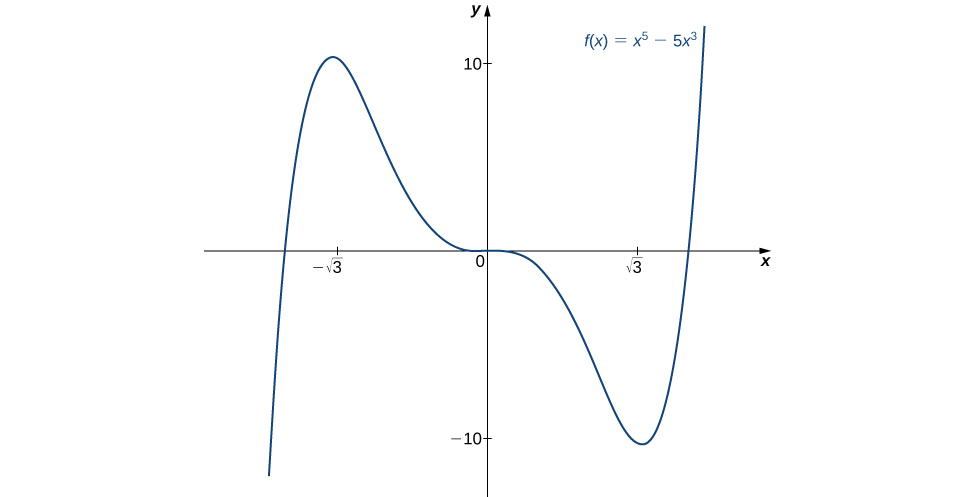
Use the second derivative to find the location of all local extrema for [latex]f(x)=x^5-5x^3[/latex].

Show Solution

To apply the second derivative test, we first need to find critical points [latex]c[/latex] where [latex]f^{\prime}(c)=0[/latex]. The derivative is [latex]f^{\prime}(x)=5x^4-15x^2[/latex]. Therefore, [latex]f^{\prime}(x)=5x^4-15x^2=5x^2(x^2-3)=0[/latex] when [latex]x=0,\pm \sqrt{3}[/latex].

To determine whether [latex]f[/latex] has a local extrema at any of these points, we need to evaluate the sign of [latex]f^{\prime \prime}[/latex] at these points. The second derivative is

[latex]f^{\prime \prime}(x)=20x^3-30x=10x(2x^2-3)[/latex].

In the following table, we evaluate the second derivative at each of the critical points and use the second derivative test to determine whether [latex]f[/latex] has a local maximum or local minimum at any of these points.

[latex]x[/latex]	[latex]f^{\prime \prime}(x)[/latex]	Conclusion
[latex]−\sqrt{3}[/latex]	[latex]-30\sqrt{3}[/latex]	Local maximum
0	0	Second derivative test is inconclusive
[latex]\sqrt{3}[/latex]	[latex]30\sqrt{3}[/latex]	Local minimum

By the second derivative test, we conclude that [latex]f[/latex] has a local maximum at [latex]x=−\sqrt{3}[/latex] and [latex]f[/latex] has a local minimum at [latex]x=\sqrt{3}[/latex]. The second derivative test is inconclusive at [latex]x=0[/latex]. To determine whether [latex]f[/latex] has a local extrema at [latex]x=0[/latex], we apply the first derivative test. To evaluate the sign of [latex]f^{\prime}(x)=5x^2(x^2-3)[/latex] for [latex]x \in (−\sqrt{3},0)[/latex] and [latex]x \in (0,\sqrt{3})[/latex], let [latex]x=-1[/latex] and [latex]x=1[/latex] be the two test points. Since [latex]f^{\prime}(-1)<0[/latex] and [latex]f^{\prime}(1)<0[/latex], we conclude that [latex]f[/latex] is decreasing on both intervals and, therefore, [latex]f[/latex] does not have a local extrema at [latex]x=0[/latex] as shown in the following graph.

Figure 10. The function [latex]f[/latex] has a local maximum at [latex]x=−\sqrt{3}[/latex] and a local minimum at [latex]x=\sqrt{3}[/latex]

Watch the following video to see the worked solution to Example: Using the Second Derivative Test.

We have now developed the tools we need to determine where a function is increasing and decreasing, as well as acquired an understanding of the basic shape of the graph. Next we discuss what happens to a function as [latex]x \to \pm \infty[/latex]. At that point, we have enough tools to provide accurate graphs of a large variety of functions.