Sketch the graph of a function that has been shifted, stretched, or reflected from its initial graph position
We have seen several cases in which we have added, subtracted, or multiplied constants to form variations of simple functions. In the previous example, for instance, we subtracted 2 from the argument of the function [latex]y=x^2[/latex] to get the function [latex]f(x)=(x-2)^2[/latex]. This subtraction represents a shift of the function [latex]y=x^2[/latex] two units to the right. A shift, horizontally or vertically, is a type of transformation of a function. Other transformations include horizontal and vertical scalings, and reflections about the axes.
Vertical Shift
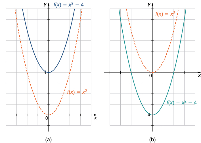
A vertical shift of a function occurs if we add or subtract the same constant to each output [latex]y[/latex]. For [latex]c>0[/latex], the graph of [latex]f(x)+c[/latex] is a shift of the graph of [latex]f(x)[/latex] up [latex]c[/latex] units, whereas the graph of [latex]f(x)-c[/latex] is a shift of the graph of [latex]f(x)[/latex] down [latex]c[/latex] units. For example, the graph of the function [latex]f(x)=x^3+4[/latex] is the graph of [latex]y=x^3[/latex] shifted up 4 units; the graph of the function [latex]f(x)=x^3-4[/latex] is the graph of [latex]y=x^3[/latex] shifted down 4 units (Figure 15).
Figure 15. (a) For [latex]c>0[/latex], the graph of [latex]y=f(x)+c[/latex] is a vertical shift up [latex]c[/latex] units of the graph of [latex]y=f(x)[/latex]. (b) For [latex]c>0[/latex], the graph of [latex]y=f(x)-c[/latex] is a vertical shift down [latex]c[/latex] units of the graph of [latex]y=f(x)[/latex].
Horizontal Shift
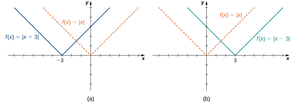
A horizontal shift of a function occurs if we add or subtract the same constant to each input [latex]x[/latex]. For [latex]c>0[/latex], the graph of [latex]f(x+c)[/latex] is a shift of the graph of [latex]f(x)[/latex] to the left [latex]c[/latex] units; the graph of [latex]f(x-c)[/latex] is a shift of the graph of [latex]f(x)[/latex] to the right [latex]c[/latex] units. Why does the graph shift left when adding a constant and shift right when subtracting a constant? To answer this question, let’s look at an example.
Consider the function [latex]f(x)=|x+3|[/latex] and evaluate this function at [latex]x-3.[/latex] Since [latex]f(x-3)=|x|[/latex] and [latex]x-3
Figure 16. (a) For [latex]c>0[/latex], the graph of [latex]y=f(x+c)[/latex] is a horizontal shift left [latex]c[/latex] units of the graph of [latex]y=f(x)[/latex]. (b) For [latex]c>0[/latex], the graph of [latex]y=f(x-c)[/latex] is a horizontal shift right [latex]c[/latex] units of the graph of [latex]y=f(x)[/latex].
Vertical Scaling (Stretched/Compressed)
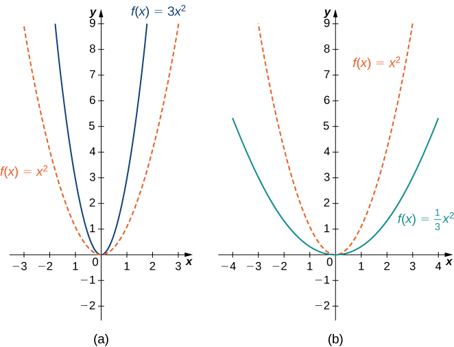
A vertical scaling of a graph occurs if we multiply all outputs [latex]y[/latex] of a function by the same positive constant. For [latex]c>0[/latex], the graph of the function [latex]cf(x)[/latex] is the graph of [latex]f(x)[/latex] scaled vertically by a factor of [latex]c[/latex]. If [latex]c>1[/latex], the values of the outputs for the function [latex]cf(x)[/latex] are larger than the values of the outputs for the function [latex]f(x)[/latex]; therefore, the graph has been stretched vertically. If [latex]0
Figure 17. (a) If [latex]c>1[/latex], the graph of [latex]y=cf(x)[/latex] is a vertical stretch of the graph of [latex]y=f(x)[/latex]. (b) If [latex]0<c<1[/latex], the graph of [latex]y=cf(x)[/latex] is a vertical compression of the graph of [latex]y=f(x)[/latex].
Horizontal Scaling (Stretched/Compressed)
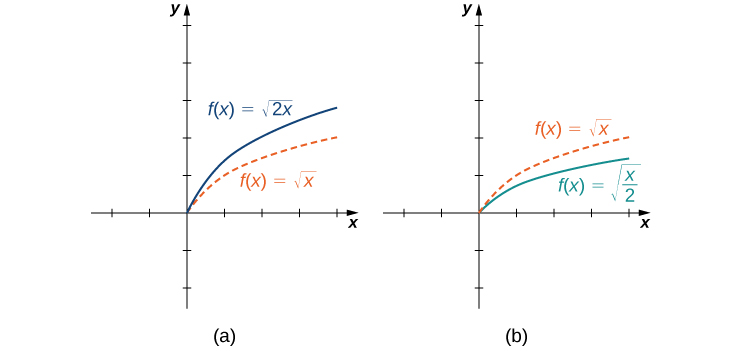
The horizontal scaling of a function occurs if we multiply the inputs [latex]x[/latex] by the same positive constant. For [latex]c>0[/latex], the graph of the function [latex]f(cx)[/latex] is the graph of [latex]f(x)[/latex] scaled horizontally by a factor of [latex]c[/latex]. If [latex]c>1[/latex], the graph of [latex]f(cx)[/latex] is the graph of [latex]f(x)[/latex] compressed horizontally. If [latex]0
Figure 18. (a) If [latex]c>1[/latex], the graph of [latex]y=f(cx)[/latex] is a horizontal compression of the graph of [latex]y=f(x)[/latex]. (b) If [latex]0<c<1[/latex], the graph of [latex]y=f(cx)[/latex] is a horizontal stretch of the graph of [latex]y=f(x)[/latex].
Reflection
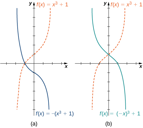
We have explored what happens to the graph of a function [latex]f[/latex] when we multiply [latex]f[/latex] by a constant [latex]c>0[/latex] to get a new function [latex]cf(x)[/latex]. We have also discussed what happens to the graph of a function [latex]f[/latex] when we multiply the independent variable [latex]x[/latex] by [latex]c>0[/latex] to get a new function [latex]f(cx)[/latex]. However, we have not addressed what happens to the graph of the function if the constant [latex]c[/latex] is negative. If we have a constant [latex]c<0[/latex], we can write [latex]c[/latex] as a positive number multiplied by [latex]-1[/latex]; but, what kind of transformation do we get when we multiply the function or its argument by [latex]-1[/latex]? When we multiply all the outputs by [latex]-1[/latex], we get a reflection about the [latex]x[/latex]-axis. When we multiply all inputs by [latex]-1[/latex], we get a reflection about the [latex]y[/latex]-axis. For example, the graph of [latex]f(x)=−(x^3+1)[/latex] is the graph of [latex]y=(x^3+1)[/latex] reflected about the [latex]x[/latex]-axis. The graph of [latex]f(x)=(−x)^3+1[/latex] is the graph of [latex]y=x^3+1[/latex] reflected about the [latex]y[/latex]-axis (Figure 19).
Figure 19. (a) The graph of [latex]y=−f(x)[/latex] is the graph of [latex]y=f(x)[/latex] reflected about the [latex]x[/latex]-axis. (b) The graph of [latex]y=f(−x)[/latex] is the graph of [latex]y=f(x)[/latex] reflected about the [latex]y[/latex]-axis.
Multiple Transformations
If the graph of a function consists of more than one transformation of another graph, it is important to transform the graph in the correct order. Given a function [latex]f(x)[/latex], the graph of the related function [latex]y=cf(a(x+b))+d[/latex] can be obtained from the graph of [latex]y=f(x)[/latex] by performing the transformations in the following order.
Horizontal shift of the graph of [latex]y=f(x)[/latex]. If [latex]b>0[/latex], shift left. If [latex]b<0[/latex], shift right.
Horizontal scaling of the graph of [latex]y=f(x+b)[/latex] by a factor of [latex]|a|[/latex]. If [latex]a<0[/latex], reflect the graph about the [latex]y[/latex]-axis.
Vertical scaling of the graph of [latex]y=f(a(x+b))[/latex] by a factor of [latex]|c|[/latex]. If [latex]c<0[/latex], reflect the graph about the [latex]x[/latex]-axis.
Vertical shift of the graph of [latex]y=cf(a(x+b))[/latex]. If [latex]d>0[/latex], shift up. If [latex]d<0[/latex], shift down.
We can summarize the different transformations and their related effects on the graph of a function in the following table.
Transformations of Functions
Transformation of [latex]f(c>0)[/latex]
Effect on the graph of[latex]f[/latex]
[latex]f(x)+c[/latex]
Vertical shift up [latex]c[/latex] units
[latex]f(x)-c[/latex]
Vertical shift down [latex]c[/latex] units
[latex]f(x+c)[/latex]
Shift left by [latex]c[/latex] units
[latex]f(x-c)[/latex]
Shift right by [latex]c[/latex] units
[latex]cf(x)[/latex]
Vertical stretch if [latex]c>1[/latex];
vertical compression if [latex]0
[latex]f(cx)[/latex]
Horizontal stretch if [latex]01[/latex]
[latex]−f(x)[/latex]
Reflection about the [latex]x[/latex]-axis
[latex]f(−x)[/latex]
Reflection about the [latex]y[/latex]-axis
Example: Transforming a Function
For each of the following functions, a. and b., sketch a graph by using a sequence of transformations of a well-known function.
[latex]f(x)=−|x+2|-3[/latex]
[latex]f(x)=3\sqrt{−x}+1[/latex]
Show Solution
Starting with the graph of [latex]y=|x|[/latex], shift 2 units to the left, reflect about the [latex]x[/latex]-axis, and then shift down 3 units.
Figure 20. The function [latex]f(x)=−|x+2|-3[/latex] can be viewed as a sequence of three transformations of the function [latex]y=|x|[/latex].
Starting with the graph of [latex]y=\sqrt{x}[/latex], reflect about the [latex]y[/latex]-axis, stretch the graph vertically by a factor of 3, and move up 1 unit.
Figure 21. The function [latex]f(x)=3\sqrt{−x}+1[/latex] can be viewed as a sequence of three transformations of the function [latex]y=\sqrt{x}[/latex].
Watch the following video to see the worked solution to Example: Transforming a Function
Closed Captioning and Transcript Information for Video
For closed captioning, open the video on its original page by clicking the Youtube logo in the lower right-hand corner of the video display. In YouTube, the video will begin at the same starting point as this clip, but will continue playing until the very end.