Graphs and Symmetry of Polar Curves

Learning Outcomes

Sketch polar curves from given equations
Convert equations between rectangular and polar coordinates
Identify symmetry in polar curves and equations

Polar Curves

Now that we know how to plot points in the polar coordinate system, we can discuss how to plot curves. In the rectangular coordinate system, we can graph a function [latex]y=f\left(x\right)[/latex] and create a curve in the Cartesian plane. In a similar fashion, we can graph a curve that is generated by a function [latex]r=f\left(\theta \right)[/latex].

The general idea behind graphing a function in polar coordinates is the same as graphing a function in rectangular coordinates. Start with a list of values for the independent variable ([latex]\theta[/latex] in this case) and calculate the corresponding values of the dependent variable [latex]r[/latex]. This process generates a list of ordered pairs, which can be plotted in the polar coordinate system. Finally, connect the points, and take advantage of any patterns that may appear. The function may be periodic, for example, which indicates that only a limited number of values for the independent variable are needed.

Problem-Solving Strategy: Plotting a Curve in Polar Coordinates

Create a table with two columns. The first column is for [latex]\theta [/latex], and the second column is for [latex]r[/latex].
Create a list of values for [latex]\theta [/latex].
Calculate the corresponding [latex]r[/latex] values for each [latex]\theta [/latex].
Plot each ordered pair [latex]\left(r,\theta \right)[/latex] on the coordinate axes.
Connect the points and look for a pattern.

Interactive

Watch this video for more information on sketching polar curves.

Example: Graphing a Function in Polar Coordinates

Graph the curve defined by the function [latex]r=4\sin\theta [/latex]. Identify the curve and rewrite the equation in rectangular coordinates.

Show Solution

Because the function is a multiple of a sine function, it is periodic with period [latex]2\pi [/latex], so use values for [latex]\theta [/latex] between 0 and [latex]2\pi [/latex]. The result of steps 1–3 appear in the following table. Figure 5 shows the graph based on this table.

[latex]\theta [/latex]	[latex]r=4\sin\theta [/latex]	[latex]\theta [/latex]	[latex]r=4\sin\theta [/latex]
[latex]0[/latex]	[latex]0[/latex]	[latex]\pi [/latex]	[latex]0[/latex]
[latex]\frac{\pi }{6}[/latex]	[latex]2[/latex]	[latex]\frac{7\pi }{6}[/latex]	[latex]-2[/latex]
[latex]\frac{\pi }{4}[/latex]	[latex]2\sqrt{2}\approx 2.8[/latex]	[latex]\frac{5\pi }{4}[/latex]	[latex]-2\sqrt{2}\approx -2.8[/latex]
[latex]\frac{\pi }{3}[/latex]	[latex]2\sqrt{3}\approx 3.4[/latex]	[latex]\frac{4\pi }{3}[/latex]	[latex]-2\sqrt{3}\approx -3.4[/latex]
[latex]\frac{\pi }{2}[/latex]	[latex]4[/latex]	[latex]\frac{3\pi }{2}[/latex]	[latex]4[/latex]
[latex]\frac{2\pi }{3}[/latex]	[latex]2\sqrt{3}\approx 3.4[/latex]	[latex]\frac{5\pi }{3}[/latex]	[latex]-2\sqrt{3}\approx -3.4[/latex]
[latex]\frac{3\pi }{4}[/latex]	[latex]2\sqrt{2}\approx 2.8[/latex]	[latex]\frac{7\pi }{4}[/latex]	[latex]-2\sqrt{2}\approx -2.8[/latex]
[latex]\frac{5\pi }{6}[/latex]	[latex]2[/latex]	[latex]\frac{11\pi }{6}[/latex]	[latex]-2[/latex]
		[latex]2\pi [/latex]	[latex]0[/latex]

On the polar coordinate plane, a circle is drawn with radius 2. It touches the origin, (2 times the square root of 2, π/4), (4, π/2), and (2 times the square root of 2, 3π/4).

This is the graph of a circle. The equation [latex]r=4\sin\theta [/latex] can be converted into rectangular coordinates by first multiplying both sides by [latex]r[/latex]. This gives the equation [latex]{r}^{2}=4r\sin\theta [/latex]. Next use the facts that [latex]{r}^{2}={x}^{2}+{y}^{2}[/latex] and [latex]y=r\sin\theta [/latex]. This gives [latex]{x}^{2}+{y}^{2}=4y[/latex]. To put this equation into standard form, subtract [latex]4y[/latex] from both sides of the equation and complete the square:

[latex]\begin{array}{ccc}\hfill {x}^{2}+{y}^{2}-4y& =\hfill & 0\hfill \\ \hfill {x}^{2}+\left({y}^{2}-4y\right)& =\hfill & 0\hfill \\ \hfill {x}^{2}+\left({y}^{2}-4y+4\right)& =\hfill & 0+4\hfill \\ \hfill {x}^{2}+{\left(y - 2\right)}^{2}& =\hfill & 4.\hfill \end{array}[/latex]

This is the equation of a circle with radius 2 and center [latex]\left(0,2\right)[/latex] in the rectangular coordinate system.

Watch the following video to see the worked solution to Example: Graphing a Function in Polar Coordinates.

For closed captioning, open the video on its original page by clicking the Youtube logo in the lower right-hand corner of the video display. In YouTube, the video will begin at the same starting point as this clip, but will continue playing until the very end.

You can view the transcript for this segmented clip of “7.3 Polar Coordinates” here (opens in new window).

try it

Create a graph of the curve defined by the function [latex]r=4+4\cos\theta [/latex].

Hint

Show Solution

The graph in the previous example was that of a circle. The equation of the circle can be transformed into rectangular coordinates using the coordinate transformation formulas in the theorem. The example after the next gives some more examples of functions for transforming from polar to rectangular coordinates.

Example: Transforming Polar Equations to Rectangular Coordinates

Rewrite each of the following equations in rectangular coordinates and identify the graph.

[latex]\theta =\frac{\pi }{3}[/latex]
[latex]r=3[/latex]
[latex]r=6\cos\theta -8\sin\theta [/latex]

Show Solution

Take the tangent of both sides. This gives [latex]\tan\theta =\tan\left(\frac{\pi}{3}\right)=\sqrt{3}[/latex]. Since [latex]\tan\theta =\frac{y}{x}[/latex] we can replace the left-hand side of this equation by [latex]\frac{y}{x}[/latex]. This gives [latex]\frac{y}{x}=\sqrt{3}[/latex], which can be rewritten as [latex]y=x\sqrt{3}[/latex]. This is the equation of a straight line passing through the origin with slope [latex]\sqrt{3}[/latex]. In general, any polar equation of the form [latex]\theta =K[/latex] represents a straight line through the pole with slope equal to [latex]\tan{K}[/latex].
First, square both sides of the equation. This gives [latex]{r}^{2}=9[/latex]. Next replace [latex]{r}^{2}[/latex] with [latex]{x}^{2}+{y}^{2}[/latex]. This gives the equation [latex]{x}^{2}+{y}^{2}=9[/latex], which is the equation of a circle centered at the origin with radius 3. In general, any polar equation of the form [latex]r=k[/latex] where k is a positive constant represents a circle of radius k centered at the origin. (Note: when squaring both sides of an equation it is possible to introduce new points unintentionally. This should always be taken into consideration. However, in this case we do not introduce new points. For example, [latex]\left(-3,\frac{\pi }{3}\right)[/latex] is the same point as [latex]\left(3,\frac{4\pi}{3}\right)[/latex].)
Multiply both sides of the equation by [latex]r[/latex]. This leads to [latex]{r}^{2}=6r\cos\theta -8r\sin\theta [/latex]. Next use the formulas

[latex]{r}^{2}={x}^{2}+{y}^{2},x=r\cos\theta ,y=r\sin\theta [/latex].

This gives

[latex]\begin{array}{ccc}\hfill {r}^{2}& =\hfill & 6\left(r\cos\theta \right)-8\left(r\sin\theta \right)\hfill \\ \hfill {x}^{2}+{y}^{2}& =\hfill & 6x - 8y.\hfill \end{array}[/latex]

To put this equation into standard form, first move the variables from the right-hand side of the equation to the left-hand side, then complete the square.

[latex]\begin{array}{ccc}\hfill {x}^{2}+{y}^{2}& =\hfill & 6x - 8y\hfill \\ \hfill {x}^{2}-6x+{y}^{2}+8y& =\hfill & 0\hfill \\ \hfill \left({x}^{2}-6x\right)+\left({y}^{2}+8y\right)& =\hfill & 0\hfill \\ \hfill \left({x}^{2}-6x+9\right)+\left({y}^{2}+8y+16\right)& =\hfill & 9+16\hfill \\ \hfill {\left(x - 3\right)}^{2}+{\left(y+4\right)}^{2}& =\hfill & 25.\hfill \end{array}[/latex]

This is the equation of a circle with center at [latex]\left(3,-4\right)[/latex] and radius 5. Notice that the circle passes through the origin since the center is 5 units away.

Watch the following video to see the worked solution to Example: Transforming Polar Equations to Rectangular Coordinates.

You can view the transcript for this segmented clip of “7.3 Polar Coordinates” here (opens in new window).

try it

Rewrite the equation [latex]r=\sec\theta \tan\theta [/latex] in rectangular coordinates and identify its graph.

Hint

Show Solution

We have now seen several examples of drawing graphs of curves defined by polar equations. A summary of some common curves is given in the tables below. In each equation, a and b are arbitrary constants.

This table has three columns and 3 rows. The first row is a header row and is given from left to right as name, equation, and example. The second row is Line passing through the pole with slope tan K; θ = K; and a picture of a straight line on the polar coordinate plane with θ = π/3. The third row is Circle; r = a cosθ + b sinθ; and a picture of a circle on the polar coordinate plane with equation r = 2 cos(t) – 3 sin(t): the circle touches the origin but has center in the third quadrant.

This table has three columns and 3 rows. The first row is Spiral; r = a + bθ; and a picture of a spiral starting at the origin with equation r = θ/3. The second row is Cardioid; r = a(1 + cosθ), r = a(1 – cosθ), r = a(1 + sinθ), r = a(1 – sinθ); and a picture of a cardioid with equation r = 3(1 + cosθ): the cardioid looks like a heart turned on its side with a rounded bottom instead of a pointed one. The third row is Limaçon; r = a cosθ + b, r = a sinθ + b; and a picture of a limaçon with equation r = 2 + 4 sinθ: the figure looks like a deformed circle with a loop inside of it. The seventh row is Rose; r = a cos(bθ), r = a sin(bθ); and a picture of a rose with equation r = 3 sin(2θ): the rose looks like a flower with four petals, one petal in each quadrant, each with length 3 and reaching to the origin between each petal.

A cardioid is a special case of a limaçon (pronounced “lee-mah-son”), in which [latex]a=b[/latex] or [latex]a=-b[/latex]. The rose is a very interesting curve. Notice that the graph of [latex]r=3\sin2\theta [/latex] has four petals. However, the graph of [latex]r=3\sin3\theta [/latex] has three petals as shown.

A rose with three petals, one in the first quadrant, another in the second quadrant, and the third in both the third and fourth quadrants, each with length 3. Each petal starts and ends at the origin.

If the coefficient of [latex]\theta [/latex] is even, the graph has twice as many petals as the coefficient. If the coefficient of [latex]\theta [/latex] is odd, then the number of petals equals the coefficient. You are encouraged to explore why this happens. Even more interesting graphs emerge when the coefficient of [latex]\theta [/latex] is not an integer. For example, if it is rational, then the curve is closed; that is, it eventually ends where it started (Figure 10 (a)). However, if the coefficient is irrational, then the curve never closes (Figure 10 (b)). Although it may appear that the curve is closed, a closer examination reveals that the petals just above the positive x axis are slightly thicker. This is because the petal does not quite match up with the starting point.

This figure has two figures. The first is a rose with so many overlapping petals that there are a few patterns that develop, starting with a sharp 10 pointed star in the center and moving out to an increasingly rounded set of petals. The second figure is a rose with even more overlapping petals, so many so that it is impossible to tell what is happening in the center, but on the outer edges are a number of sharply rounded petals.

Since the curve defined by the graph of [latex]r=3\sin\left(\pi \theta \right)[/latex] never closes, the curve depicted in Figure 10 (b) is only a partial depiction. In fact, this is an example of a space-filling curve. A space-filling curve is one that in fact occupies a two-dimensional subset of the real plane. In this case the curve occupies the circle of radius 3 centered at the origin.

Suppose a curve is described in the polar coordinate system via the function [latex]r=f\left(\theta \right)[/latex]. Since we have conversion formulas from polar to rectangular coordinates given by

[latex]\begin{array}{c}x=r\cos\theta \hfill \\ y=r\sin\theta ,\hfill \end{array}[/latex]

it is possible to rewrite these formulas using the function

[latex]\begin{array}{c}x=f\left(\theta \right)\cos\theta \hfill \\ y=f\left(\theta \right)\sin\theta .\hfill \end{array}[/latex]

This step gives a parameterization of the curve in rectangular coordinates using [latex]\theta [/latex] as the parameter. For example, the spiral formula [latex]r=a+b\theta [/latex] from Figure 7 becomes

[latex]\begin{array}{c}x=\left(a+b\theta \right)\cos\theta \hfill \\ y=\left(a+b\theta \right)\sin\theta .\hfill \end{array}[/latex]

Letting [latex]\theta [/latex] range from [latex]-\infty [/latex] to [latex]\infty [/latex] generates the entire spiral.

Try It

Symmetry in Polar Coordinates

When studying symmetry of functions in rectangular coordinates (i.e., in the form [latex]y=f\left(x\right)[/latex]), we talk about symmetry with respect to the y-axis and symmetry with respect to the origin. In particular, if [latex]f\left(-x\right)=f\left(x\right)[/latex] for all [latex]x[/latex] in the domain of [latex]f[/latex], then [latex]f[/latex] is an even function and its graph is symmetric with respect to the [latex]y[/latex]-axis. If [latex]f\left(-x\right)=-f\left(x\right)[/latex] for all [latex]x[/latex] in the domain of [latex]f[/latex], then [latex]f[/latex] is an odd function and its graph is symmetric with respect to the origin. By determining which types of symmetry a graph exhibits, we can learn more about the shape and appearance of the graph. Symmetry can also reveal other properties of the function that generates the graph. Symmetry in polar curves works in a similar fashion.

theorem: Symmetry in Polar Curves and Equations

Consider a curve generated by the function [latex]r=f\left(\theta \right)[/latex] in polar coordinates.

The curve is symmetric about the polar axis if for every point [latex]\left(r,\theta \right)[/latex] on the graph, the point [latex]\left(r,-\theta \right)[/latex] is also on the graph. Similarly, the equation [latex]r=f\left(\theta \right)[/latex] is unchanged by replacing [latex]\theta [/latex] with [latex]-\theta [/latex].
The curve is symmetric about the pole if for every point [latex]\left(r,\theta \right)[/latex] on the graph, the point [latex]\left(r,\pi +\theta \right)[/latex] is also on the graph. Similarly, the equation [latex]r=f\left(\theta \right)[/latex] is unchanged when replacing [latex]r[/latex] with [latex]-r[/latex], or [latex]\theta [/latex] with [latex]\pi +\theta [/latex].
The curve is symmetric about the vertical line [latex]\theta =\frac{\pi }{2}[/latex] if for every point [latex]\left(r,\theta \right)[/latex] on the graph, the point [latex]\left(r,\pi -\theta \right)[/latex] is also on the graph. Similarly, the equation [latex]r=f\left(\theta \right)[/latex] is unchanged when [latex]\theta [/latex] is replaced by [latex]\pi -\theta [/latex].

The following table shows examples of each type of symmetry.

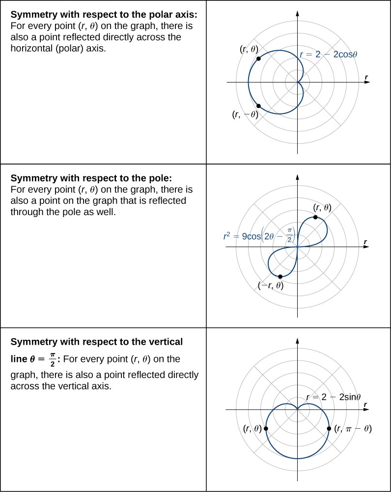
This table has three rows and two columns. The first row reads

Figure 11.

Example: using Symmetry to Graph a Polar Equation

Find the symmetry of the rose defined by the equation [latex]r=3\sin\left(2\theta \right)[/latex] and create a graph.

Show Solution

Suppose the point [latex]\left(r,\theta \right)[/latex] is on the graph of [latex]r=3\sin\left(2\theta \right)[/latex].

To test for symmetry about the polar axis, first try replacing [latex]\theta [/latex] with [latex]-\theta [/latex]. This gives [latex]r=3\sin\left(2\left(-\theta \right)\right)=-3\sin\left(2\theta \right)[/latex]. Since this changes the original equation, this test is not satisfied. However, returning to the original equation and replacing [latex]r[/latex] with [latex]-r[/latex] and [latex]\theta [/latex] with [latex]\pi -\theta [/latex] yields

[latex]\begin{array}{}\\ -r=3\sin\left(2\left(\pi -\theta \right)\right)\hfill \\ -r=3\sin\left(2\pi -2\theta \right)\hfill \\ -r=3\sin\left(-2\theta \right)\hfill \\ -r=-3\sin2\theta .\hfill \end{array}[/latex]

Multiplying both sides of this equation by [latex]-1[/latex] gives [latex]r=3\sin2\theta [/latex], which is the original equation. This demonstrates that the graph is symmetric with respect to the polar axis.
To test for symmetry with respect to the pole, first replace [latex]r[/latex] with [latex]-r[/latex], which yields [latex]-r=3\sin\left(2\theta \right)[/latex]. Multiplying both sides by −1 gives [latex]r=-3\sin\left(2\theta \right)[/latex], which does not agree with the original equation. Therefore the equation does not pass the test for this symmetry. However, returning to the original equation and replacing [latex]\theta [/latex] with [latex]\theta +\pi [/latex] gives

[latex]\begin{array}{cc}\hfill r& =3\sin\left(2\left(\theta +\pi \right)\right)\hfill \\ & =3\sin\left(2\theta +2\pi \right)\hfill \\ & =3\left(\sin2\theta \cos2\pi +\cos2\theta \sin2\pi \right)\hfill \\ & =3\sin2\theta .\hfill \end{array}[/latex]

Since this agrees with the original equation, the graph is symmetric about the pole.
To test for symmetry with respect to the vertical line [latex]\theta =\frac{\pi }{2}[/latex], first replace both [latex]r[/latex] with [latex]-r[/latex] and [latex]\theta [/latex] with [latex]-\theta [/latex].

[latex]\begin{array}{}\\ -r=3\sin\left(2\left(-\theta \right)\right)\hfill \\ -r=3\sin\left(-2\theta \right)\hfill \\ -r=-3\sin2\theta .\hfill \end{array}[/latex]

Multiplying both sides of this equation by [latex]-1[/latex] gives [latex]r=3\sin2\theta [/latex], which is the original equation. Therefore the graph is symmetric about the vertical line [latex]\theta =\frac{\pi }{2}[/latex].

This graph has symmetry with respect to the polar axis, the origin, and the vertical line going through the pole. To graph the function, tabulate values of [latex]\theta [/latex] between 0 and [latex]\frac{\pi}{2}[/latex] and then reflect the resulting graph.

[latex]\theta [/latex]	[latex]r[/latex]
[latex]0[/latex]	[latex]0[/latex]
[latex]\frac{\pi }{6}[/latex]	[latex]\frac{3\sqrt{3}}{2}\approx 2.6[/latex]
[latex]\frac{\pi }{4}[/latex]	[latex]3[/latex]
[latex]\frac{\pi }{3}[/latex]	[latex]\frac{3\sqrt{3}}{2}\approx 2.6[/latex]
[latex]\frac{\pi }{2}[/latex]	[latex]0[/latex]

This gives one petal of the rose, as shown in the following graph.

A single petal is graphed with equation r = 3 sin(2θ) for 0 ≤ θ ≤ π/2. It starts at the origin and reaches a maximum distance from the origin of 3.

Reflecting this image into the other three quadrants gives the entire graph as shown.

A four-petaled rose is graphed with equation r = 3 sin(2θ). Each petal starts at the origin and reaches a maximum distance from the origin of 3.

Watch the following video to see the worked solution to Example: using Symmetry to Graph a Polar Equation.

You can view the transcript for this segmented clip of “7.3 Polar Coordinates” here (opens in new window).

try it

Determine the symmetry of the graph determined by the equation [latex]r=2\cos\left(3\theta \right)[/latex] and create a graph.

Hint

Show Solution

Module 7: Parametric Equations and Polar Coordinates