Usually a given differential equation has an infinite number of solutions, so it is natural to ask which one we want to use. To choose one solution, more information is needed. Some specific information that can be useful is an initial value, which is an ordered pair that is used to find a particular solution.

A differential equation together with one or more initial values is called an initial-value problem. The general rule is that the number of initial values needed for an initial-value problem is equal to the order of the differential equation. For example, if we have the differential equation [latex]{y}^{\prime }=2x[/latex], then [latex]y\left(3\right)=7[/latex] is an initial value, and when taken together, these equations form an initial-value problem. The differential equation [latex]y\text{''}-3{y}^{\prime }+2y=4{e}^{x}[/latex] is second order, so we need two initial values. With initial-value problems of order greater than one, the same value should be used for the independent variable. An example of initial values for this second-order equation would be [latex]y\left(0\right)=2[/latex] and [latex]{y}^{\prime }\left(0\right)=-1[/latex]. These two initial values together with the differential equation form an initial-value problem. These problems are so named because often the independent variable in the unknown function is [latex]t[/latex], which represents time. Thus, a value of [latex]t=0[/latex] represents the beginning of the problem.

Watch the following video to see the worked solution to Example: Verifying a Solution to an Initial-Value Problem

For closed captioning, open the video on its original page by clicking the Youtube logo in the lower right-hand corner of the video display. In YouTube, the video will begin at the same starting point as this clip, but will continue playing until the very end.

You can view the transcript for this segmented clip of “4.1.5” here (opens in new window).

In the previous example, the initial-value problem consisted of two parts. The first part was the differential equation [latex]{y}^{\prime }+2y=3{e}^{x}[/latex], and the second part was the initial value [latex]y\left(0\right)=3[/latex]. These two equations together formed the initial-value problem.

The same is true in general. An initial-value problem will consists of two parts: the differential equation and the initial condition. The differential equation has a family of solutions, and the initial condition determines the value of [latex]C[/latex]. The family of solutions to the differential equation in the example is given by [latex]y=2{e}^{-2t}+C{e}^{t}[/latex]. This family of solutions is shown in Figure 2, with the particular solution [latex]y=2{e}^{-2t}+{e}^{t}[/latex] labeled.

Figure 2. A family of solutions to the differential equation [latex]{y}^{\prime }+2y=3{e}^{t}[/latex]. The particular solution [latex]y=2{e}^{-2t}+{e}^{t}[/latex] is labeled.

Watch the following video to see the worked solution to Example: Verifying a Solution to an Initial-Value Problem

For closed captioning, open the video on its original page by clicking the Youtube logo in the lower right-hand corner of the video display. In YouTube, the video will begin at the same starting point as this clip, but will continue playing until the very end.

You can view the transcript for this segmented clip of “4.1.5” here (opens in new window).

In physics and engineering applications, we often consider the forces acting upon an object, and use this information to understand the resulting motion that may occur. For example, if we start with an object at Earth’s surface, the primary force acting upon that object is gravity. Physicists and engineers can use this information, along with Newton’s second law of motion (in equation form [latex]F=ma[/latex], where [latex]F[/latex] represents force, [latex]m[/latex] represents mass, and [latex]a[/latex] represents acceleration), to derive an equation that can be solved.

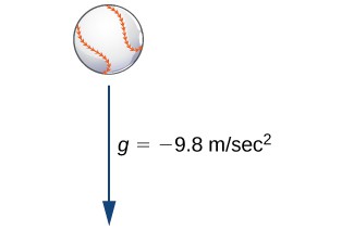
Figure 3. For a baseball falling in air, the only force acting on it is gravity (neglecting air resistance).

In Figure 3. we assume that the only force acting on a baseball is the force of gravity. This assumption ignores air resistance. (The force due to air resistance is considered in a later discussion.) The acceleration due to gravity at Earth’s surface, [latex]g[/latex], is approximately [latex]9.8{\text{m/s}}^{2}[/latex]. We introduce a frame of reference, where Earth’s surface is at a height of 0 meters. Let [latex]v\left(t\right)[/latex] represent the velocity of the object in meters per second. If [latex]v\left(t\right)>0[/latex], the ball is rising, and if [latex]v\left(t\right)<0[/latex], the ball is falling (Figure 4).

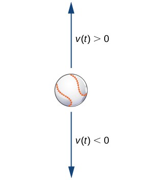
Figure 4. Possible velocities for the rising/falling baseball.

Our goal is to solve for the velocity [latex]v\left(t\right)[/latex] at any time [latex]t[/latex]. To do this, we set up an initial-value problem. Suppose the mass of the ball is [latex]m[/latex], where [latex]m[/latex] is measured in kilograms. We use Newton’s second law, which states that the force acting on an object is equal to its mass times its acceleration [latex]\left(F=ma\right)[/latex]. Acceleration is the derivative of velocity, so [latex]a\left(t\right)={v}^{\prime }\left(t\right)[/latex]. Therefore the force acting on the baseball is given by [latex]F=m{v}^{\prime }\left(t\right)[/latex]. However, this force must be equal to the force of gravity acting on the object, which (again using Newton’s second law) is given by [latex]{F}_{g}=\text{-}mg[/latex], since this force acts in a downward direction. Therefore we obtain the equation [latex]F={F}_{g}[/latex], which becomes [latex]m{v}^{\prime }\left(t\right)=\text{-}mg[/latex]. Dividing both sides of the equation by [latex]m[/latex] gives the equation

 

Notice that this differential equation remains the same regardless of the mass of the object.

We now need an initial value. Because we are solving for velocity, it makes sense in the context of the problem to assume that we know the initial velocity, or the velocity at time [latex]t=0[/latex]. This is denoted by [latex]v\left(0\right)={v}_{0}[/latex].

A natural question to ask after solving this type of problem is how high the object will be above Earth’s surface at a given point in time. Let [latex]s\left(t\right)[/latex] denote the height above Earth’s surface of the object, measured in meters. Because velocity is the derivative of position (in this case height), this assumption gives the equation [latex]{s}^{\prime }\left(t\right)=v\left(t\right)[/latex]. An initial value is necessary; in this case the initial height of the object works well. Let the initial height be given by the equation [latex]s\left(0\right)={s}_{0}[/latex]. Together these assumptions give the initial-value problem

 

If the velocity function is known, then it is possible to solve for the position function as well.