Learning Outcomes
- Calculate the limit of a sequence if it exists
A fundamental question that arises regarding infinite sequences is the behavior of the terms as [latex]n[/latex] gets larger. Since a sequence is a function defined on the positive integers, it makes sense to discuss the limit of the terms as [latex]n\to \infty[/latex]. For example, consider the following four sequences and their different behaviors as [latex]n\to \infty[/latex] (see Figure 2):
- [latex]\left\{1+3n\right\}=\left\{4,7,10,13\text{,}\ldots\right\}[/latex]. The terms [latex]1+3n[/latex] become arbitrarily large as [latex]n\to \infty[/latex]. In this case, we say that [latex]1+3n\to \infty[/latex] as [latex]n\to \infty[/latex].
- [latex]\left\{1-{\left(\frac{1}{2}\right)}^{n}\right\}=\left\{\frac{1}{2},\frac{3}{4},\frac{7}{8},\frac{15}{16}\text{,}\ldots\right\}[/latex]. The terms [latex]1-{\left(\frac{1}{2}\right)}^{n}\to 1[/latex] as [latex]n\to \infty[/latex].
- [latex]\left\{{\left(-1\right)}^{n}\right\}=\left\{\text{-}1,1,-1,1\text{,}\ldots\right\}[/latex]. The terms alternate but do not approach one single value as [latex]n\to \infty[/latex].
- [latex]\left\{\frac{{\left(-1\right)}^{n}}{n}\right\}=\left\{-1,\frac{1}{2},-\frac{1}{3},\frac{1}{4}\text{,}\ldots\right\}[/latex]. The terms alternate for this sequence as well, but [latex]\frac{{\left(-1\right)}^{n}}{n}\to 0[/latex] as [latex]n\to \infty[/latex].
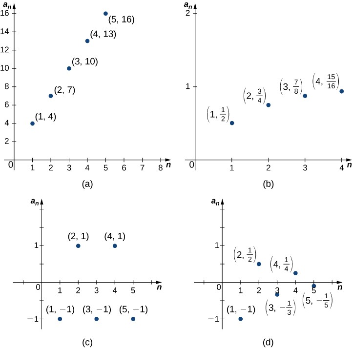
Figure 2. (a) The terms in the sequence become arbitrarily large as [latex]n\to \infty [/latex]. (b) The terms in the sequence approach [latex]1[/latex] as [latex]n\to \infty [/latex]. (c) The terms in the sequence alternate between [latex]1[/latex] and [latex]-1[/latex] as [latex]n\to \infty [/latex]. (d) The terms in the sequence alternate between positive and negative values but approach [latex]0[/latex] as [latex]n\to \infty [/latex].
From these examples, we see several possibilities for the behavior of the terms of a sequence as [latex]n\to \infty[/latex]. In two of the sequences, the terms approach a finite number as [latex]n\to \infty[/latex]. In the other two sequences, the terms do not. If the terms of a sequence approach a finite number [latex]L[/latex] as [latex]n\to \infty[/latex], we say that the sequence is a convergent sequence and the real number [latex]L[/latex] is the limit of the sequence. We can give an informal definition here.
Definition
Given a sequence [latex]\left\{{a}_{n}\right\}[/latex], if the terms [latex]{a}_{n}[/latex] become arbitrarily close to a finite number [latex]L[/latex] as [latex]n[/latex] becomes sufficiently large, we say [latex]\left\{{a}_{n}\right\}[/latex] is a convergent sequence and [latex]L[/latex] is the limit of the sequence. In this case, we write
If a sequence [latex]\left\{{a}_{n}\right\}[/latex] is not convergent, we say it is a divergent sequence.
From Figure 2, we see that the terms in the sequence [latex]\left\{1-{\left(\frac{1}{2}\right)}^{n}\right\}[/latex] are becoming arbitrarily close to [latex]1[/latex] as [latex]n[/latex] becomes very large. We conclude that [latex]\left\{1-{\left(\frac{1}{2}\right)}^{n}\right\}[/latex] is a convergent sequence and its limit is [latex]1[/latex]. In contrast, from Figure 2, we see that the terms in the sequence [latex]1+3n[/latex] are not approaching a finite number as [latex]n[/latex] becomes larger. We say that [latex]\left\{1+3n\right\}[/latex] is a divergent sequence.
In the informal definition for the limit of a sequence, we used the terms “arbitrarily close” and “sufficiently large.” Although these phrases help illustrate the meaning of a converging sequence, they are somewhat vague. To be more precise, we now present the more formal definition of limit for a sequence and show these ideas graphically in Figure 3.
Definition
A sequence [latex]\left\{{a}_{n}\right\}[/latex] converges to a real number [latex]L[/latex] if for all [latex]\epsilon >0[/latex], there exists an integer [latex]N[/latex] such that [latex]|{a}_{n}-L|<\epsilon[/latex] if [latex]n\ge N[/latex]. The number [latex]L[/latex] is the limit of the sequence and we write
In this case, we say the sequence [latex]\left\{{a}_{n}\right\}[/latex] is a convergent sequence. If a sequence does not converge, it is a divergent sequence, and we say the limit does not exist.
We remark that the convergence or divergence of a sequence [latex]\left\{{a}_{n}\right\}[/latex] depends only on what happens to the terms [latex]{a}_{n}[/latex] as [latex]n\to \infty[/latex]. Therefore, if a finite number of terms [latex]{b}_{1},{b}_{2}\text{,}\ldots,{b}_{N}[/latex] are placed before [latex]{a}_{1}[/latex] to create a new sequence
this new sequence will converge if [latex]\left\{{a}_{n}\right\}[/latex] converges and diverge if [latex]\left\{{a}_{n}\right\}[/latex] diverges. Further, if the sequence [latex]\left\{{a}_{n}\right\}[/latex] converges to [latex]L[/latex], this new sequence will also converge to [latex]L[/latex].
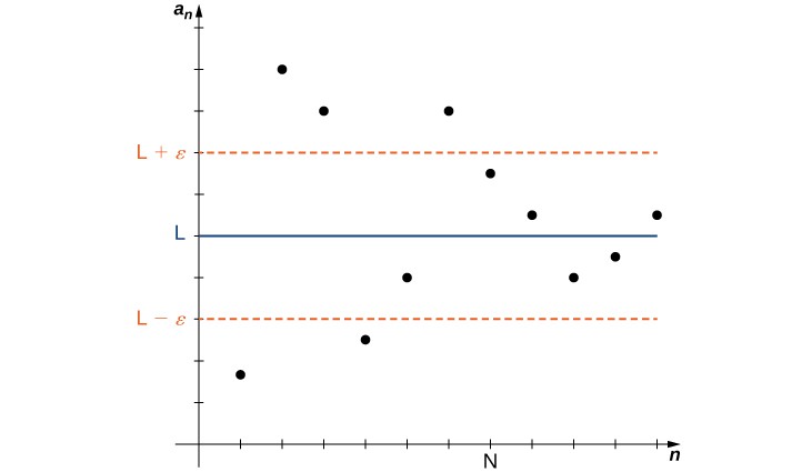
Figure 3. As [latex]n[/latex] increases, the terms [latex]{a}_{n}[/latex] become closer to [latex]L[/latex]. For values of [latex]n\ge N[/latex], the distance between each point [latex]\left(n,{a}_{n}\right)[/latex] and the line [latex]y=L[/latex] is less than [latex]\epsilon [/latex].
As defined above, if a sequence does not converge, it is said to be a divergent sequence. For example, the sequences [latex]\left\{1+3n\right\}[/latex] and [latex]\left\{{\left(-1\right)}^{n}\right\}[/latex] shown in Figure 3 diverge. However, different sequences can diverge in different ways. The sequence [latex]\left\{{\left(-1\right)}^{n}\right\}[/latex] diverges because the terms alternate between [latex]1[/latex] and [latex]-1[/latex], but do not approach one value as [latex]n\to \infty[/latex]. On the other hand, the sequence [latex]\left\{1+3n\right\}[/latex] diverges because the terms [latex]1+3n\to \infty[/latex] as [latex]n\to \infty[/latex]. We say the sequence [latex]\left\{1+3n\right\}[/latex] diverges to infinity and write [latex]\underset{n\to \infty }{\text{lim}}\left(1+3n\right)=\infty[/latex]. It is important to recognize that this notation does not imply the limit of the sequence [latex]\left\{1+3n\right\}[/latex] exists. The sequence is, in fact, divergent. Writing that the limit is infinity is intended only to provide more information about why the sequence is divergent. A sequence can also diverge to negative infinity. For example, the sequence [latex]\left\{\text{-}5n+2\right\}[/latex] diverges to negative infinity because [latex]-5n+2\to \text{-}\infty[/latex] as [latex]n\to \text{-}\infty[/latex]. We write this as [latex]\underset{n\to \infty }{\text{lim}}\left(-5n+2\right)=\to \text{-}\infty[/latex].
Because a sequence is a function whose domain is the set of positive integers, we can use properties of limits of functions to determine whether a sequence converges. For example, consider a sequence [latex]\left\{{a}_{n}\right\}[/latex] and a related function [latex]f[/latex] defined on all positive real numbers such that [latex]f\left(n\right)={a}_{n}[/latex] for all integers [latex]n\ge 1[/latex]. Since the domain of the sequence is a subset of the domain of [latex]f[/latex], if [latex]\underset{x\to \infty }{\text{lim}}f\left(x\right)[/latex] exists, then the sequence converges and has the same limit. For example, consider the sequence [latex]\left\{\frac{1}{n}\right\}[/latex] and the related function [latex]f\left(x\right)=\frac{1}{x}[/latex]. Since the function [latex]f[/latex] defined on all real numbers [latex]x>0[/latex] satisfies [latex]f\left(x\right)=\frac{1}{x}\to 0[/latex] as [latex]x\to \infty[/latex], the sequence [latex]\left\{\frac{1}{n}\right\}[/latex] must satisfy [latex]\frac{1}{n}\to 0[/latex] as [latex]n\to \infty[/latex].
Theorem: Limit of a Sequence Defined by a Function
Consider a sequence [latex]\left\{{a}_{n}\right\}[/latex] such that [latex]{a}_{n}=f\left(n\right)[/latex] for all [latex]n\ge 1[/latex]. If there exists a real number [latex]L[/latex] such that
then [latex]\left\{{a}_{n}\right\}[/latex] converges and
We can use this theorem to evaluate [latex]\underset{n\to \infty }{\text{lim}}{r}^{n}[/latex] for [latex]0\le r\le 1[/latex]. For example, consider the sequence [latex]\left\{{\left(\frac{1}{2}\right)}^{n}\right\}[/latex] and the related exponential function [latex]f\left(x\right)={\left(\frac{1}{2}\right)}^{x}[/latex]. Since [latex]\underset{x\to \infty }{\text{lim}}{\left(\frac{1}{2}\right)}^{x}=0[/latex], we conclude that the sequence [latex]\left\{{\left(\frac{1}{2}\right)}^{n}\right\}[/latex] converges and its limit is [latex]0[/latex]. Similarly, for any real number [latex]r[/latex] such that [latex]0\le r<1[/latex], [latex]\underset{x\to \infty }{\text{lim}}{r}^{x}=0[/latex], and therefore the sequence [latex]\left\{{r}^{n}\right\}[/latex] converges. On the other hand, if [latex]r=1[/latex], then [latex]\underset{x\to \infty }{\text{lim}}{r}^{x}=1[/latex], and therefore the limit of the sequence [latex]\left\{{1}^{n}\right\}[/latex] is [latex]1[/latex]. If [latex]r>1[/latex], [latex]\underset{x\to \infty }{\text{lim}}{r}^{x}=\infty[/latex], and therefore we cannot apply this theorem. However, in this case, just as the function [latex]{r}^{x}[/latex] grows without bound as [latex]n\to \infty[/latex], the terms [latex]{r}^{n}[/latex] in the sequence become arbitrarily large as [latex]n\to \infty[/latex], and we conclude that the sequence [latex]\left\{{r}^{n}\right\}[/latex] diverges to infinity if [latex]r>1[/latex].
We summarize these results regarding the geometric sequence [latex]\left\{{r}^{n}\right\}\text{:}[/latex]
Later in this section we consider the case when [latex]r<0[/latex].
We now consider slightly more complicated sequences. For example, consider the sequence [latex]\left\{{\left(\frac{2}{3}\right)}^{n}+{\left(\frac{1}{4}\right)}^{n}\right\}[/latex]. The terms in this sequence are more complicated than other sequences we have discussed, but luckily the limit of this sequence is determined by the limits of the two sequences [latex]\left\{{\left(\frac{2}{3}\right)}^{n}\right\}[/latex] and [latex]\left\{{\left(\frac{1}{4}\right)}^{n}\right\}[/latex]. As we describe in the following algebraic limit laws, since [latex]\left\{{\left(\frac{2}{3}\right)}^{n}\right\}[/latex] and[latex]\left\{{\left(\frac{1}{4}\right)}^{n}\right\}[/latex] both converge to [latex]0[/latex], the sequence [latex]\left\{{\left(\frac{2}{3}\right)}^{n}+{\left(\frac{1}{4}\right)}^{n}\right\}[/latex] converges to [latex]0+0=0[/latex]. Just as we were able to evaluate a limit involving an algebraic combination of functions [latex]f[/latex] and [latex]g[/latex] by looking at the limits of [latex]f[/latex] and [latex]g[/latex] (see Introduction to Limits), we are able to evaluate the limit of a sequence whose terms are algebraic combinations of [latex]{a}_{n}[/latex] and [latex]{b}_{n}[/latex] by evaluating the limits of [latex]\left\{{a}_{n}\right\}[/latex] and [latex]\left\{{b}_{n}\right\}[/latex].
Theorem: Algebraic Limit Laws
Given sequences [latex]\left\{{a}_{n}\right\}[/latex] and [latex]\left\{{b}_{n}\right\}[/latex] and any real number [latex]c[/latex], if there exist constants [latex]A[/latex] and [latex]B[/latex] such that [latex]\underset{n\to \infty }{\text{lim}}{a}_{n}=A[/latex] and [latex]\underset{n\to \infty }{\text{lim}}{b}_{n}=B[/latex], then
- [latex]\underset{n\to \infty }{\text{lim}}c=c[/latex]
- [latex]\underset{n\to \infty }{\text{lim}}c{a}_{n}=c\underset{n\to \infty }{\text{lim}}{a}_{n}=cA[/latex]
- [latex]\underset{n\to \infty }{\text{lim}}\left({a}_{n}\pm {b}_{n}\right)=\underset{n\to \infty }{\text{lim}}{a}_{n}\pm \underset{n\to \infty }{\text{lim}}{b}_{n}=A\pm B[/latex]
- [latex]\underset{\text{n}\to \infty }{\text{lim}}\left({a}_{n}\cdot {b}_{n}\right)=\left(\underset{n\to \infty }{\text{lim}}{a}_{n}\right)\cdot \left(\underset{n\to \infty }{\text{lim}}{b}_{n}\right)=A\cdot B[/latex]
- [latex]\underset{n\to \infty }{\text{lim}}\left(\frac{{a}_{n}}{{b}_{n}}\right)=\frac{\underset{n\to \infty }{\text{lim}}{a}_{n}}{\underset{n\to \infty }{\text{lim}}{b}_{n}}=\frac{A}{B}[/latex], provided [latex]B\ne 0[/latex] and each [latex]{b}_{n}\ne 0[/latex].
Proof
We prove part iii.
Let [latex]>0[/latex]. Since [latex]\underset{n\to \infty }{\text{lim}}{a}_{n}=A[/latex], there exists a constant positive integer [latex]{N}_{1}[/latex] such that for all [latex]n\ge {N}_{1}[/latex]. Since [latex]\underset{n\to \infty }{\text{lim}}{b}_{n}=B[/latex], there exists a constant [latex]{N}_{2}[/latex] such that [latex]|{b}_{n}-B|<\frac{\epsilon}{2}[/latex] for all [latex]n\ge {N}_{2}[/latex]. Let [latex]N[/latex] be the largest of [latex]{N}_{1}[/latex] and [latex]{N}_{2}[/latex]. Therefore, for all [latex]n\ge N[/latex],
[latex]|\left({a}_{n}+{b}_{n}\right)\text{-}\left(A+B\right)|\le |{a}_{n}-A|+|{b}_{n}-B|<\frac{\epsilon }{2}+\frac{\epsilon }{2}=\epsilon[/latex].
[latex]_\blacksquare[/latex]
The algebraic limit laws allow us to evaluate limits for many sequences. For example, consider the sequence [latex]\left\{\frac{1}{{n}^{2}}\right\}[/latex]. As shown earlier, [latex]\underset{n\to \infty }{\text{lim}}\frac{1}{n}=0[/latex]. Similarly, for any positive integer [latex]k[/latex], we can conclude that
In the next example, we make use of this fact along with the limit laws to evaluate limits for other sequences. First, we revisit a principle from precalculus for evaluating the end behavior of rational functions that will help with one such example
Recall: End Behavior of Rational Functions
The value of [latex]\lim_{x \to \infty} \frac{P(x)}{Q(x)}[/latex], where [latex]P(x)[/latex] and [latex]Q(x)[/latex] are polynomials can be determined by looking at the degrees of the numerator and denominator.
- Case 1: If the degree of [latex]P(x)[/latex] is less than the degree of [latex]Q(x)[/latex]: [latex]\lim_{x \to \infty} \frac{P(x)}{Q(x)} = 0[/latex]
- Case 2: If the degree of [latex]P(x)[/latex] is greater than the degree of [latex]Q(x)[/latex]: [latex]\lim_{x \to \infty} \frac{P(x)}{Q(x)} = \infty[/latex] (or [latex]-\infty[/latex])
- Case 3: If the degree of [latex]P(x)[/latex] is equal to the degree of [latex]Q(x)[/latex]: [latex]\lim_{x \to \infty} \frac{P(x)}{Q(x)} = \frac{p}{q}[/latex], the ratio of the leading coefficients of [latex]P(x)[/latex] and [latex]Q(x)[/latex], respectively.
Example: Determining Convergence and Finding Limits
For each of the following sequences, determine whether or not the sequence converges. If it converges, find its limit.
- [latex]\left\{5-\frac{3}{{n}^{2}}\right\}[/latex]
- [latex]\left\{\frac{3{n}^{4}-7{n}^{2}+5}{6 - 4{n}^{4}}\right\}[/latex]
- [latex]\left\{\frac{{2}^{n}}{{n}^{2}}\right\}[/latex]
- [latex]\left\{{\left(1+\frac{4}{n}\right)}^{n}\right\}[/latex]
We will often explore the behavior of sequences featuring a ratio of terms where both numerator and denominator are increasing without bound and it is not immediately apparent what the ratio of these terms will be as the input grows unboundedly large. To find the limit of such expressions, we can use L’Hôpital’s Rule.
Recall: L’Hôpital’s Rule
Suppose [latex]f[/latex] and [latex]g[/latex] are differentiable functions over an open interval [latex]\left(a, \infty \right)[/latex] for some value of [latex]a[/latex]. If either:
- [latex]\underset{x\to \infty}{\lim}f(x)=0[/latex] and [latex]\underset{x\to \infty}{\lim}g(x)=0[/latex]
- [latex]\underset{x\to \infty}{\lim}f(x)= \infty[/latex] (or [latex]-\infty[/latex]) and [latex]\underset{x\to \infty}{\lim}g(x)= \infty[/latex] (or [latex]-\infty[/latex]), then
assuming the limit on the right exists or is [latex]\infty[/latex] or [latex]−\infty[/latex].
try it
Consider the sequence [latex]\left\{\frac{\left(5{n}^{2}+1\right)}{{e}^{n}}\right\}[/latex]. Determine whether or not the sequence converges. If it converges, find its limit.
Watch the following video to see the worked solution to the above Try IT.
For closed captioning, open the video on its original page by clicking the Youtube logo in the lower right-hand corner of the video display. In YouTube, the video will begin at the same starting point as this clip, but will continue playing until the very end.
You can view the transcript for this segmented clip of “5.1.2” here (opens in new window).
Recall that if [latex]f[/latex] is a continuous function at a value [latex]L[/latex], then [latex]f\left(x\right)\to f\left(L\right)[/latex] as [latex]x\to L[/latex]. This idea applies to sequences as well. Suppose a sequence [latex]{a}_{n}\to L[/latex], and a function [latex]f[/latex] is continuous at [latex]L[/latex]. Then [latex]f\left({a}_{n}\right)\to f\left(L\right)[/latex]. This property often enables us to find limits for complicated sequences. For example, consider the sequence [latex]\sqrt{5-\frac{3}{{n}^{2}}}[/latex]. From the previous example. we know the sequence [latex]5-\frac{3}{{n}^{2}}\to 5[/latex]. Since [latex]\sqrt{x}[/latex] is a continuous function at [latex]x=5[/latex],
Theorem: Continuous Functions Defined on Convergent Sequences
Consider a sequence [latex]\left\{{a}_{n}\right\}[/latex] and suppose there exists a real number [latex]L[/latex] such that the sequence [latex]\left\{{a}_{n}\right\}[/latex] converges to [latex]L[/latex]. Suppose [latex]f[/latex] is a continuous function at [latex]L[/latex]. Then there exists an integer [latex]N[/latex] such that [latex]f[/latex] is defined at all values [latex]{a}_{n}[/latex] for [latex]n\ge N[/latex], and the sequence [latex]\left\{f\left({a}_{n}\right)\right\}[/latex] converges to [latex]f\left(L\right)[/latex].
Proof
Let [latex]>0[/latex]. Since [latex]f[/latex] is continuous at [latex]L[/latex], there exists [latex]\delta >0[/latex] such that [latex]|f\left(x\right)-f\left(L\right)|<\epsilon[/latex] if [latex]|x-L|<\delta[/latex]. Since the sequence [latex]\left\{{a}_{n}\right\}[/latex] converges to [latex]L[/latex], there exists [latex]N[/latex] such that [latex]|{a}_{n}-L|<\delta[/latex] for all [latex]n\ge N[/latex]. Therefore, for all [latex]n\ge N[/latex], [latex]|{a}_{n}-L|<\delta[/latex], which implies [latex]|f\left({a}_{n}\right)\text{-}f\left(L\right)|<\epsilon[/latex]. We conclude that the sequence [latex]\left\{f\left({a}_{n}\right)\right\}[/latex] converges to [latex]f\left(L\right)[/latex].
[latex]_\blacksquare[/latex]
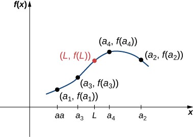
Figure 4. Because [latex]f[/latex] is a continuous function as the inputs [latex]{a}_{1},{a}_{2},{a}_{3}\text{,}\ldots[/latex] approach [latex]L[/latex], the outputs [latex]f\left({a}_{1}\right),f\left({a}_{2}\right),f\left({a}_{3}\right)\text{,}\ldots[/latex] approach [latex]f\left(L\right)[/latex].
Example: Limits Involving Continuous Functions Defined on Convergent Sequences
Determine whether the sequence [latex]\left\{\cos\left(\frac{3}{{n}^{2}}\right)\right\}[/latex] converges. If it converges, find its limit.
try it
Determine if the sequence [latex]\left\{\sqrt{\frac{2n+1}{3n+5}}\right\}[/latex] converges. If it converges, find its limit.
Watch the following video to see the worked solution to the above Try IT.
For closed captioning, open the video on its original page by clicking the Youtube logo in the lower right-hand corner of the video display. In YouTube, the video will begin at the same starting point as this clip, but will continue playing until the very end.
You can view the transcript for this segmented clip of “5.1.2” here (opens in new window).
Another theorem involving limits of sequences is an extension of the Squeeze Theorem for limits discussed in Introduction to Limits.
Theorem: Squeeze Theorem for Sequences
Consider sequences [latex]\left\{{a}_{n}\right\}[/latex], [latex]\left\{{b}_{n}\right\}[/latex], and [latex]\left\{{c}_{n}\right\}[/latex]. Suppose there exists an integer [latex]N[/latex] such that
If there exists a real number [latex]L[/latex] such that
then [latex]\left\{{b}_{n}\right\}[/latex] converges and [latex]\underset{n\to \infty }{\text{lim}}{b}_{n}=L[/latex] (Figure 5).
Proof
Let [latex]\epsilon >0[/latex]. Since the sequence [latex]\left\{{a}_{n}\right\}[/latex] converges to [latex]L[/latex], there exists an integer [latex]{N}_{1}[/latex] such that [latex]|{a}_{n}-L|<\epsilon[/latex] for all [latex]n\ge {N}_{1}[/latex]. Similarly, since [latex]\left\{{c}_{n}\right\}[/latex] converges to [latex]L[/latex], there exists an integer [latex]{N}_{2}[/latex] such that [latex]|{c}_{n}-L|<\epsilon[/latex] for all [latex]n\ge {N}_{2}[/latex]. By assumption, there exists an integer [latex]N[/latex] such that [latex]{a}_{n}\le {b}_{n}\le {c}_{n}[/latex] for all [latex]n\ge N[/latex]. Let [latex]M[/latex] be the largest of [latex]{N}_{1},{N}_{2}[/latex], and [latex]N[/latex]. We must show that [latex]|{b}_{n}-L|<\epsilon[/latex] for all [latex]n\ge M[/latex]. For all [latex]n\ge M[/latex],
Therefore, [latex]\text{-}\epsilon <{b}_{n}-L<\epsilon[/latex], and we conclude that [latex]|{b}_{n}-L|<\epsilon[/latex] for all [latex]n\ge M[/latex], and we conclude that the sequence [latex]\left\{{b}_{n}\right\}[/latex] converges to [latex]L[/latex].
[latex]_\blacksquare[/latex]
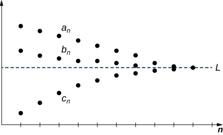
Figure 5. Each term [latex]{b}_{n}[/latex] satisfies [latex]{a}_{n}\le {b}_{n}\le {c}_{n}[/latex] and the sequences [latex]\left\{{a}_{n}\right\}[/latex] and [latex]\left\{{c}_{n}\right\}[/latex] converge to the same limit, so the sequence [latex]\left\{{b}_{n}\right\}[/latex] must converge to the same limit as well.
Example: Using the Squeeze theorem
Use the Squeeze Theorem to find the limit of each of the following sequences.
- [latex]\left\{\frac{\cos{n}}{{n}^{2}}\right\}[/latex]
- [latex]\left\{{\left(-\frac{1}{2}\right)}^{n}\right\}[/latex]
try it
Find [latex]\underset{n\to \infty }{\text{lim}}\frac{2n-\sin{n}}{n}[/latex].
Watch the following video to see the worked solution to the above Try IT.
For closed captioning, open the video on its original page by clicking the Youtube logo in the lower right-hand corner of the video display. In YouTube, the video will begin at the same starting point as this clip, but will continue playing until the very end.
You can view the transcript for this segmented clip of “5.1.2” here (opens in new window).
Using the idea from the previous example, we conclude that [latex]{r}^{n}\to 0[/latex] for any real number [latex]r[/latex] such that [latex]-1
Candela Citations
- 5.1.2. Authored by: Ryan Melton. License: CC BY: Attribution
- Calculus Volume 2. Authored by: Gilbert Strang, Edwin (Jed) Herman. Provided by: OpenStax. Located at: https://openstax.org/books/calculus-volume-2/pages/1-introduction. License: CC BY-NC-SA: Attribution-NonCommercial-ShareAlike. License Terms: Access for free at https://openstax.org/books/calculus-volume-2/pages/1-introduction
