Learning Outcomes
- Determine the mass of a one-dimensional object from its linear density function
- Determine the mass of a two-dimensional circular object from its radial density function
We can use integration to develop a formula for calculating mass based on a density function. First we consider a thin rod or wire. Orient the rod so it aligns with the [latex]x\text{-axis,}[/latex] with the left end of the rod at [latex]x=a[/latex] and the right end of the rod at [latex]x=b[/latex] (Figure 1). Note that although we depict the rod with some thickness in the figures, for mathematical purposes we assume the rod is thin enough to be treated as a one-dimensional object.
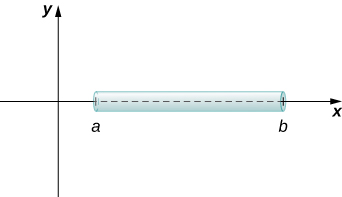
Figure 1. We can calculate the mass of a thin rod oriented along the [latex]x\text{-axis}[/latex] by integrating its density function.
If the rod has constant density [latex]\rho ,[/latex] given in terms of mass per unit length, then the mass of the rod is just the product of the density and the length of the rod: [latex](b-a)\rho .[/latex] If the density of the rod is not constant, however, the problem becomes a little more challenging. When the density of the rod varies from point to point, we use a linear density function, [latex]\rho (x),[/latex] to denote the density of the rod at any point, [latex]x.[/latex] Let [latex]\rho (x)[/latex] be an integrable linear density function. Now, for [latex]i=0,1,2\text{,…},n[/latex] let [latex]P=\left\{{x}_{i}\right\}[/latex] be a regular partition of the interval [latex]\left[a,b\right],[/latex] and for [latex]i=1,2\text{,…},n[/latex] choose an arbitrary point [latex]{x}_{i}^{*}\in \left[{x}_{i-1},{x}_{i}\right].[/latex] Figure 2 shows a representative segment of the rod.
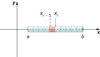
Figure 2. A representative segment of the rod.
The mass [latex]{m}_{i}[/latex] of the segment of the rod from [latex]{x}_{i-1}[/latex] to [latex]{x}_{i}[/latex] is approximated by
Adding the masses of all the segments gives us an approximation for the mass of the entire rod:
This is a Riemann sum. Taking the limit as [latex]n\to \infty ,[/latex] we get an expression for the exact mass of the rod:
We state this result in the following theorem.
Mass–Density Formula of a One-Dimensional Object
Given a thin rod oriented along the [latex]x\text{-axis}[/latex] over the interval [latex]\left[a,b\right],[/latex] let [latex]\rho (x)[/latex] denote a linear density function giving the density of the rod at a point [latex]x[/latex] in the interval. Then the mass of the rod is given by
We apply this theorem in the next example.
Example: Calculating Mass from Linear Density
Consider a thin rod oriented on the [latex]x[/latex]-axis over the interval [latex]\left[\frac{\pi}{2},\pi \right].[/latex] If the density of the rod is given by [latex]\rho (x)= \sin x,[/latex] what is the mass of the rod?
Try It
Consider a thin rod oriented on the [latex]x[/latex]-axis over the interval [latex]\left[1,3\right].[/latex] If the density of the rod is given by [latex]\rho (x)=2{x}^{2}+3,[/latex] what is the mass of the rod?
Watch the following video to see the worked solution to the above Try It.
Try It
We now extend this concept to find the mass of a two-dimensional disk of radius [latex]r.[/latex] As with the rod we looked at in the one-dimensional case, here we assume the disk is thin enough that, for mathematical purposes, we can treat it as a two-dimensional object. We assume the density is given in terms of mass per unit area (called area density), and further assume the density varies only along the disk’s radius (called radial density). We orient the disk in the [latex]xy\text{-plane,}[/latex] with the center at the origin. Then, the density of the disk can be treated as a function of [latex]x,[/latex] denoted [latex]\rho (x).[/latex] We assume [latex]\rho (x)[/latex] is integrable. Because density is a function of [latex]x,[/latex] we partition the interval from [latex]\left[0,r\right][/latex] along the [latex]x\text{-axis}.[/latex] For [latex]i=0,1,2\text{,…},n,[/latex] let [latex]P=\left\{{x}_{i}\right\}[/latex] be a regular partition of the interval [latex]\left[0,r\right],[/latex] and for [latex]i=1,2\text{,…},n,[/latex] choose an arbitrary point [latex]{x}_{i}^{*}\in \left[{x}_{i-1},{x}_{i}\right].[/latex] Now, use the partition to break up the disk into thin (two-dimensional) washers. A disk and a representative washer are depicted in the following figure.
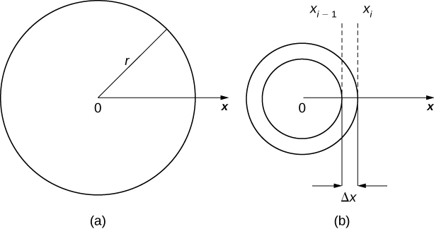
Figure 3. (a) A thin disk in the xy-plane. (b) A representative washer.
We now approximate the density and area of the washer to calculate an approximate mass, [latex]{m}_{i}.[/latex] Note that the area of the washer is given by
You may recall that we had an expression similar to this when we were computing volumes by shells. As we did there, we use [latex]{x}_{i}^{*}\approx ({x}_{i}+{x}_{i-1})\text{/}2[/latex] to approximate the average radius of the washer. We obtain
Using [latex]\rho ({x}_{i}^{*})[/latex] to approximate the density of the washer, we approximate the mass of the washer by
Adding up the masses of the washers, we see the mass [latex]m[/latex] of the entire disk is approximated by
We again recognize this as a Riemann sum, and take the limit as [latex]n\to \infty .[/latex] This gives us
We summarize these findings in the following theorem.
Mass–Density Formula of a Circular Object
Let [latex]\rho (x)[/latex] be an integrable function representing the radial density of a disk of radius [latex]r.[/latex] Then the mass of the disk is given by
Example: Calculating Mass from Radial Density
Let [latex]\rho (x)=\sqrt{x}[/latex] represent the radial density of a disk. Calculate the mass of a disk of radius 4.
Try It
Let [latex]\rho (x)=3x+2[/latex] represent the radial density of a disk. Calculate the mass of a disk of radius 2.
Watch the following video to see the worked solution to the above Try It.
Candela Citations
- 2.5 Physical Applications. Authored by: Ryan Melton. License: CC BY: Attribution
- Calculus Volume 2. Authored by: Gilbert Strang, Edwin (Jed) Herman. Provided by: OpenStax. Located at: https://openstax.org/books/calculus-volume-2/pages/1-introduction. License: CC BY-NC-SA: Attribution-NonCommercial-ShareAlike. License Terms: Access for free at https://openstax.org/books/calculus-volume-2/pages/1-introduction
