Learning Outcomes
- Describe the concept of environmental carrying capacity in the logistic model of population growth
To model population growth using a differential equation, we first need to introduce some variables and relevant terms. The variable [latex]t[/latex]. will represent time. The units of time can be hours, days, weeks, months, or even years. Any given problem must specify the units used in that particular problem. The variable [latex]P[/latex] will represent population. Since the population varies over time, it is understood to be a function of time. Therefore we use the notation [latex]P\left(t\right)[/latex] for the population as a function of time. If [latex]P\left(t\right)[/latex] is a differentiable function, then the first derivative [latex]\frac{dP}{dt}[/latex] represents the instantaneous rate of change of the population as a function of time.
In Exponential Growth and Decay, we studied the exponential growth and decay of populations and radioactive substances. An example of an exponential growth function is [latex]P\left(t\right)={P}_{0}{e}^{rt}[/latex]. In this function, [latex]P\left(t\right)[/latex] represents the population at time [latex]t,{P}_{0}[/latex] represents the initial population (population at time [latex]t=0[/latex]), and the constant [latex]r>0[/latex] is called the growth rate. Figure 1 shows a graph of [latex]P\left(t\right)=100{e}^{0.03t}[/latex]. Here [latex]{P}_{0}=100[/latex] and [latex]r=0.03[/latex].
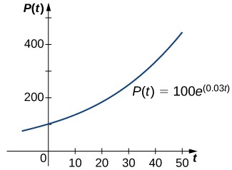
Figure 1. An exponential growth model of population.
We can verify that the function [latex]P\left(t\right)={P}_{0}{e}^{rt}[/latex] satisfies the initial-value problem
This differential equation has an interesting interpretation. The left-hand side represents the rate at which the population increases (or decreases). The right-hand side is equal to a positive constant multiplied by the current population. Therefore the differential equation states that the rate at which the population increases is proportional to the population at that point in time. Furthermore, it states that the constant of proportionality never changes.
One problem with this function is its prediction that as time goes on, the population grows without bound. This is unrealistic in a real-world setting. Various factors limit the rate of growth of a particular population, including birth rate, death rate, food supply, predators, and so on. The growth constant [latex]r[/latex] usually takes into consideration the birth and death rates but none of the other factors, and it can be interpreted as a net (birth minus death) percent growth rate per unit time. A natural question to ask is whether the population growth rate stays constant, or whether it changes over time. Biologists have found that in many biological systems, the population grows until a certain steady-state population is reached. This possibility is not taken into account with exponential growth. However, the concept of carrying capacity allows for the possibility that in a given area, only a certain number of a given organism or animal can thrive without running into resource issues.
Definition
The carrying capacity of an organism in a given environment is defined to be the maximum population of that organism that the environment can sustain indefinitely.
We use the variable [latex]K[/latex] to denote the carrying capacity. The growth rate is represented by the variable [latex]r[/latex]. Using these variables, we can define the logistic differential equation.
Definition
Let [latex]K[/latex] represent the carrying capacity for a particular organism in a given environment, and let [latex]r[/latex] be a real number that represents the growth rate. The function [latex]P\left(t\right)[/latex] represents the population of this organism as a function of time [latex]t[/latex], and the constant [latex]{P}_{0}[/latex] represents the initial population (population of the organism at time [latex]t=0[/latex]). Then the logistic differential equation is
Interactive
The logistic equation was first published by Pierre Verhulst in [latex]1845[/latex]. This differential equation can be coupled with the initial condition [latex]P\left(0\right)={P}_{0}[/latex] to form an initial-value problem for [latex]P\left(t\right)[/latex].
Suppose that the initial population is small relative to the carrying capacity. Then [latex]\frac{P}{K}[/latex] is small, possibly close to zero. Thus, the quantity in parentheses on the right-hand side of the definition is close to [latex]1[/latex], and the right-hand side of this equation is close to [latex]rP[/latex]. If [latex]r>0[/latex], then the population grows rapidly, resembling exponential growth.
However, as the population grows, the ratio [latex]\frac{P}{K}[/latex] also grows, because [latex]K[/latex] is constant. If the population remains below the carrying capacity, then [latex]\frac{P}{K}[/latex] is less than [latex]1[/latex], so [latex]1-\frac{P}{K}>0[/latex]. Therefore the right-hand side of the definition is still positive, but the quantity in parentheses gets smaller, and the growth rate decreases as a result. If [latex]P=K[/latex] then the right-hand side is equal to zero, and the population does not change.
Now suppose that the population starts at a value higher than the carrying capacity. Then [latex]\frac{P}{K}>1[/latex], and [latex]1-\frac{P}{K}<0[/latex]. Then the right-hand side of the definition is negative, and the population decreases. As long as [latex]P>K[/latex], the population decreases. It never actually reaches [latex]K[/latex] because [latex]\frac{dP}{dt}[/latex] will get smaller and smaller, but the population approaches the carrying capacity as [latex]t[/latex] approaches infinity. This analysis can be represented visually by way of a phase line. A phase line describes the general behavior of a solution to an autonomous differential equation, depending on the initial condition. For the case of a carrying capacity in the logistic equation, the phase line is as shown in Figure 2.
Figure 2. A phase line for the differential equation [latex]\frac{dP}{dt}=rP\left(1-\frac{P}{K}\right)[/latex].
This phase line shows that when [latex]P[/latex] is less than zero or greater than [latex]K[/latex], the population decreases over time. When [latex]P[/latex] is between [latex]0[/latex] and [latex]K[/latex], the population increases over time.
Example: Examining the Carrying Capacity of a Woodpecker Population
There were an estimated [latex]150[/latex] pileated woodpeckers (Dryocopus pileatus) in a forest at the beginning of 2020. At the beginning of 2021, the population had increased to about [latex]175[/latex]. Based on the size of the forest, the carrying capacity is estimated to be about [latex]400[/latex] pileated woodpeckers.
- Write a logistic differential equation and initial condition to model this population. Use [latex]t=0[/latex] for the beginning of 2020.
- Draw a direction field for this logistic differential equation, and sketch the solution curve corresponding to the initial condition.
- Solve the initial-value problem for [latex]P\left(t\right)[/latex].
- According to this model, what will the population be at the beginning of 2025?
- How long will it take the population to reach [latex]75%[/latex] of the carrying capacity?

Candela Citations
- Calculus Volume 2. Authored by: Gilbert Strang, Edwin (Jed) Herman. Provided by: OpenStax. Located at: https://openstax.org/books/calculus-volume-2/pages/1-introduction. License: CC BY-NC-SA: Attribution-NonCommercial-ShareAlike. License Terms: Access for free at https://openstax.org/books/calculus-volume-2/pages/1-introduction
