Chapter Opener: Examining the Carrying Capacity of a Deer Population

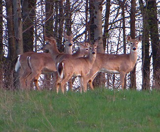
(credit: modification of work by Rachel Kramer, Flickr)

Let’s consider the population of white-tailed deer (Odocoileus virginianus) in the state of Kentucky. The Kentucky Department of Fish and Wildlife Resources (KDFWR) sets guidelines for hunting and fishing in the state. Before the hunting season of $2004$, it estimated a population of $900,000$ deer. Johnson notes: “A deer population that has plenty to eat and is not hunted by humans or other predators will double every three years.” (George Johnson, “The Problem of Exploding Deer Populations Has No Attractive Solutions,” January $12,2001$, accessed April 9, 2015, http://www.txtwriter.com/onscience/Articles/deerpops.html.) This observation corresponds to a rate of increase $r=\frac{\text{ln}\left(2\right)}{3}=0.2311$, so the approximate growth rate is $23.11\text{%}$ per year. (This assumes that the population grows exponentially, which is reasonable––at least in the short term––with plentiful food supply and no predators.) The KDFWR also reports deer population densities for $32$ counties in Kentucky, the average of which is approximately $27$ deer per square mile. Suppose this is the deer density for the whole state ($39,732$ square miles). The carrying capacity $K$ is $39,732$ square miles times $27$ deer per square mile, or $1,072,764$ deer.

1. For this application, we have ${P}_{0}=900,000,K=1,072,764$, and $r=0.2311$. Substitute these values into the logistic differential equation and form the initial-value problem.
2. Solve the initial-value problem from part a.
3. According to this model, what will be the population in $3$ years? Recall that the doubling time predicted by Johnson for the deer population was $3$ years. How do these values compare?
4. Suppose the population managed to reach $1,200,000$ deer. What does the logistic equation predict will happen to the population in this scenario?

Show Solution

1. The initial value problem is
   
   $\frac{dP}{dt}=0.2311P\left(1-\frac{P}{1,072,764}\right),P\left(0\right)=900,000$.
2. The logistic equation is an autonomous differential equation, so we can use the method of separation of variables.
   
   Step 1: Setting the right-hand side equal to zero gives $P=0$ and $P=1,072,764$. This means that if the population starts at zero it will never change, and if it starts at the carrying capacity, it will never change.
   
   Step 2: Rewrite the differential equation and multiply both sides by:
   
   $\begin{array}{ccc}\hfill \frac{dP}{dt}& =\hfill & 0.2311P\left(\frac{1,072,764-P}{1,072,764}\right)\hfill \\ \hfill dP& =\hfill & 0.2311P\left(\frac{1,072,764-P}{1,072,764}\right)dt.\hfill \end{array}$

   
   
   Divide both sides by $P\left(1,072,764-P\right)\text{:}$
   

   $\frac{dP}{P\left(1,072,764-P\right)}=\frac{0.2311}{1,072,764}dt$.

   
   
   Step 3: Integrate both sides of the equation using partial fraction decomposition:
   

   $\begin{array}{ccc}\hfill {\displaystyle\int \frac{dP}{P\left(1,072,764-P\right)}}& =\hfill & {\displaystyle\int \frac{0.2311}{1,072,764}dt}\hfill \\ \hfill \frac{1}{1,072,764}{\displaystyle\int \left(\frac{1}{P}+\frac{1}{1,072,764-P}\right)dP}& =\hfill & \frac{0.2311t}{1,072,764}+C\hfill \\ \hfill \frac{1}{1,072,764}\left(\text{ln}|P|-\text{ln}|1,072,764-P|\right)& =\hfill & \frac{0.2311t}{1,072,764}+C.\hfill \end{array}$

   
   
   Step 4: Multiply both sides by $1,072,764$ and use the quotient rule for logarithms:
   

   $\text{ln}|\frac{P}{1,072,764-P}|=0.2311t+{C}_{1}$.

   
   
   Here ${C}_{1}=1,072,764C$. Next exponentiate both sides and eliminate the absolute value:
   

   $\begin{array}{ccc}\hfill {e}^{\text{ln}|\frac{P}{1,072,764-P}|}& =\hfill & {e}^{0.2311t+{C}_{1}}\hfill \\ \hfill |\frac{P}{1,072,764-P}|& =\hfill & {C}_{2}{e}^{0.2311t}\hfill \\ \hfill \frac{P}{1,072,764-P}& =\hfill & {C}_{2}{e}^{0.2311t}.\hfill \end{array}$

   
   
   Here ${C}_{2}={e}^{{C}_{1}}$ but after eliminating the absolute value, it can be negative as well. Now solve for:
   

   $\begin{array}{ccc}\hfill P& =\hfill & {C}_{2}{e}^{0.2311t}\left(1,072,764-P\right).\hfill \\ \hfill P& =\hfill & 1,072,764{C}_{2}{e}^{0.2311t}-{C}_{2}P{e}^{0.2311t}\hfill \\ \hfill P+{C}_{2}P{e}^{0.2311t}& =\hfill & 1,072,764{C}_{2}{e}^{0.2311t}\hfill \\ \hfill P\left(1+{C}_{2}{e}^{0.2311t}\right)& =\hfill & 1,072,764{C}_{2}{e}^{0.2311t}\hfill \\ \hfill P\left(t\right)& =\hfill & \frac{1,072,764{C}_{2}{e}^{0.2311t}}{1+{C}_{2}{e}^{0.2311t}}.\hfill \end{array}$

   
   
   Step 5: To determine the value of ${C}_{2}$, it is actually easier to go back a couple of steps to where ${C}_{2}$ was defined. In particular, use the equation
   

   $\frac{P}{1,072,764-P}={C}_{2}{e}^{0.2311t}$.

   
   
   The initial condition is $P\left(0\right)=900,000$. Replace $P$ with $900,000$ and $t$ with zero:
   

   $\begin{array}{ccc}\hfill \frac{P}{1,072,764-P}& =\hfill & {C}_{2}{e}^{0.2311t}\hfill \\ \hfill \frac{900,000}{1,072,764 - 900,000}& =\hfill & {C}_{2}{e}^{0.2311\left(0\right)}\hfill \\ \hfill \frac{900,000}{172,764}& =\hfill & {C}_{2}\hfill \\ \hfill {C}_{2}& =\hfill & \frac{25,000}{4,799}\approx 5.209.\hfill \end{array}$

   
   
   Therefore
   

   $\begin{array}{cc}\hfill P\left(t\right)& =\frac{1,072,764\left(\frac{25000}{4799}\right){e}^{0.2311t}}{1+\left(\frac{25000}{4799}\right){e}^{0.2311t}}\hfill \\ & =\frac{1,072,764\left(25000\right){e}^{0.2311t}}{4799+25000{e}^{0.2311t}}.\hfill \end{array}$

   
   
   Dividing the numerator and denominator by $25,000$ gives
   

   $P\left(t\right)=\frac{1,072,764{e}^{0.2311t}}{0.19196+{e}^{0.2311t}}$.

   
   
   The graph below depicts this equation.
   

   

   Logistic curve for the deer population with an initial population of $900,000$ deer.

3. Using this model we can predict the population in $3$ years.
   
   $P\left(3\right)=\frac{1,072,764{e}^{0.2311\left(3\right)}}{0.19196+{e}^{0.2311\left(3\right)}}\approx 978,830\text{ deer}$

   
   
   This is far short of twice the initial population of $900,000$. Remember that the doubling time is based on the assumption that the growth rate never changes, but the logistic model takes this possibility into account.

4. If the population reached $1,200,000$ deer, then the new initial-value problem would be
   
   $\frac{dP}{dt}=0.2311P\left(1-\frac{P}{1,072,764}\right),P\left(0\right)=1,200,000$.

   
   
   The general solution to the differential equation would remain the same.
   

   $P\left(t\right)=\frac{1,072,764{C}_{2}{e}^{0.2311t}}{1+{C}_{2}{e}^{0.2311t}}$

   
   
   To determine the value of the constant, return to the equation
   

   $\frac{P}{1,072,764-P}={C}_{2}{e}^{0.2311t}$.

   
   
   Substituting the values $t=0$ and $P=1,200,000$, you get
   

   $\begin{array}{ccc}\hfill {C}_{2}{e}^{0.2311\left(0\right)}& =\hfill & \frac{1,200,000}{1,072,764 - 1,200,000}\hfill \\ \hfill {C}_{2}& =\hfill & -\frac{100,000}{10,603}\approx -9.431.\hfill \end{array}$

   
   
   Therefore
   

   $\begin{array}{cc}\hfill P\left(t\right)& =\frac{1,072,764{C}_{2}{e}^{0.2311t}}{1+{C}_{2}{e}^{0.2311t}}\hfill \\ & =\frac{1,072,764\left(-\frac{100,000}{10,603}\right){e}^{0.2311t}}{1+\left(-\frac{100,000}{10,603}\right){e}^{0.2311t}}\hfill \\ & =-\frac{107,276,400,000{e}^{0.2311t}}{100,000{e}^{0.2311t}-10,603}\hfill \\ & \approx \frac{10,117,551{e}^{0.2311t}}{9.43129{e}^{0.2311t}-1}.\hfill \end{array}$

   
   
   This equation is graphed below.
   

   

   Logistic curve for the deer population with an initial population of $1,200,000$ deer.

 

Watch the following video to see the worked solution to Chapter Opener: Examining the Carrying Capacity of a Deer Population

You can view the transcript for “4.4.3” here (opens in new window).

Now that we have the solution to the initial-value problem, we can choose values for ${P}_{0},r$, and $K$ and study the solution curve. Above, we used the values $r=0.2311,K=1,072,764$, and an initial population of $900,000$ deer. This leads to the solution $\begin{array}{cc}\hfill P\left(t\right)& =\dfrac{{P}_{0}K{e}^{rt}}{\left(K-{P}_{0}\right)+{P}_{0}{e}^{rt}}\hfill \\ \\ & =\dfrac{900,000\left(1,072,764\right){e}^{0.2311t}}{\left(1,072,764 - 900,000\right)+900,000{e}^{0.2311t}}\hfill \\ \\ & =\dfrac{900,000\left(1,072,764\right){e}^{0.2311t}}{172,764+900,000{e}^{0.2311t}}.\hfill \end{array}$
 

Dividing top and bottom by $900,000$ gives

This is the same as the original solution. The graph of this solution is shown again in blue in Figure 3, superimposed over the graph of the exponential growth model with initial population $900,000$ and growth rate $0.2311$ (appearing in green). The red dashed line represents the carrying capacity, and is a horizontal asymptote for the solution to the logistic equation.

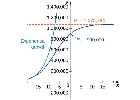
Figure 3. A comparison of exponential versus logistic growth for the same initial population of $900,000$ organisms and growth rate of $23.11\text{%}$.

Working under the assumption that the population grows according to the logistic differential equation, this graph predicts that approximately $20$ years earlier $\left(1984\right)$, the growth of the population was very close to exponential. The net growth rate at that time would have been around $23.1\text{%}$ per year. As time goes on, the two graphs separate. This happens because the population increases, and the logistic differential equation states that the growth rate decreases as the population increases. At the time the population was measured $\left(2004\right)$, it was close to carrying capacity, and the population was starting to level off.