Double Integrals over Rectangular Regions

Learning Objectives

Recognize when a function of two variables is integrable over a rectangular region.
Recognize and use some of the properties of double integrals.

Volumes and Double Integrals

We first begin with a review of the definition of the definite integral in terms of the limit of a Riemann Sum from single-variable calculus.

Recall: Riemann SumS and the Definite Integral

Suppose that [latex]y = f(x)[/latex] is a continuous function and [latex]f(x) \ge 0[/latex] on a closed interval [latex][a,b][/latex]. The area under the curve and above the [latex]y-[/latex]axis can be approximated using rectangles, by subdividing the interval [latex][a,b][/latex] into [latex]n[/latex] subintervals of width [latex]\Delta x = \frac{b-a}{n}[/latex]. If [latex]x_i[/latex] denotes a sample point within the [latex]i^{th}[/latex] subinterval, then [latex]f(x_i^\ast)[/latex] gives the height of the [latex]i^{th}[/latex] rectangle. Adding up each of these areas yields an approximation of the total area, called a Riemann Sum and denoted using the following:

[latex]\sum_{i=1}^n f(x_i^\ast)\Delta x[/latex]

The definite integral of [latex]f(x)[/latex] on [latex][a,b][/latex] represents the exact area under the curve [latex]y = f(x)[/latex], and is defined in terms as the following limit.

[latex]\int_a^b f(x)dx = \lim_{n\rightarrow\infty}\sum_{i=1}^n f(x_i^\ast)\Delta x[/latex]

To extend this notion into another dimension, we consider the space above a rectangular region [latex]R[/latex]. Consider a continuous function [latex]{f(x,y)\geq 0}[/latex] of two variables defined on the closed rectangle [latex]R[/latex]:

[latex]\large{R = [a,b]\times[c,d] = \left \{(x,y)\in {\mathbb{R}}^2 |a\leq x\leq b,c\leq y\leq d \right \}}[/latex]

Here [latex]{{[a,b]}{\times}{[c,d]}}[/latex] denotes the Cartesian product of the two closed intervals [latex]{[a,b]}[/latex] and [latex]{[c,d]}[/latex]. It consists of rectangular pairs [latex](x, y)[/latex] such that [latex]a\leq x\leq b[/latex] and [latex]c\leq y\leq d[/latex]. The graph of [latex]f[/latex] represents a surface above the [latex]xy[/latex]-plane with equation [latex]z=f(x, y)[/latex] where [latex]z[/latex] is the height of the surface at the point [latex](x, y)[/latex]. Let [latex]S[/latex] be the solid that lies above [latex]R[/latex] and under the graph of [latex]f[/latex] (Figure 1). The base of the solid is the rectangle [latex]R[/latex] in the [latex]xy[/latex]-plane. We want to find the volume [latex]V[/latex] of the solid [latex]S[/latex].

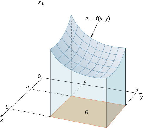
In xyz space, there is a surface z = f(x, y). On the x axis, the lines denoting a and b are drawn; on the y axis the lines for c and d are drawn. When the surface is projected onto the xy plane, it forms a rectangle with corners (a, c), (a, d), (b, c), and (b, d).

Figure 1. The graph of [latex]f(x,y)[/latex] over the rectangle [latex]R[/latex] in the [latex]xy[/latex]-plane is a curved surface.

We divide the region [latex]R[/latex] into small rectangles [latex]{R_{ij}}[/latex], each with area [latex]{\Delta{A}}[/latex] and with sides [latex]{\Delta{x}}[/latex] and [latex]{\Delta{y}}[/latex] (Figure 2). We do this by dividing the interval [latex]{[a,b]}[/latex] into [latex]m[/latex] subintervals and dividing the interval [latex]{[c,d]}[/latex] into [latex]n[/latex] subintervals. Hence [latex]{{\Delta{x}}={\dfrac{b-a}{m}},{\Delta{y}}={\dfrac{d-c}{n}},}[/latex] and [latex]{{\Delta{A}}={\Delta{x}}{\Delta{y}}}[/latex].

In the xy plane, there is a rectangle with corners (a, c), (a, d), (b, c), and (b, d). Between a and b on the x axis lines are drawn from a, x1, x2, …, xi, …, b with distance Delta x between each line; between c and d on the y axis lines are drawn from c, y1, y2, …, yj, …, d with distance Delta y between each line. Among the resulting subrectangles, the one in the second column and third row up has a point marked (x*23, y*23). The rectangle Rij is marked with upper right corner (xi, yj). Within this rectangle the point (x*ij, y*ij) is marked.

Figure 2. Rectangle [latex]R[/latex] is divided into small rectangles [latex]R_{ij}[/latex], each with an area [latex]\Delta{A}[/latex].

The volume of a thin rectangular box above [latex]{R_{ij}}[/latex] is [latex]{f{({x{_{ij}^*}},{y{_{ij}^*}})}}{\Delta{A}}[/latex], where [latex]{({x{_{ij}^*}},{y{_{ij}^*}})}[/latex] is an arbitrary sample point in each [latex]{R_{ij}}[/latex] as shown in the following figure.

Figure 3. A thin rectangular box above [latex]R_{ij}[/latex] with height [latex]f(x^{\ast}_{ij},y^{\ast}_{ij})[/latex].

Using the same idea for all the subrectangles, we obtain an approximate volume of the solid [latex]S[/latex] as [latex]{V}{\approx} \displaystyle\sum_{i=1}^{m}\sum_{j=1}^{n}\ {f{({x{_{ij}^*}},{y{_{ij}^*}})}{\Delta{A}}}[/latex]. This sum is known as a double Riemann sum and can be used to approximate the value of the volume of the solid. Here the double sum means that for each subrectangle we evaluate the function at the chosen point, multiply by the area of each rectangle, and then add all the results.

As we have seen in the single-variable case, we obtain a better approximation to the actual volume if [latex]m[/latex] and [latex]n[/latex] become larger.

[latex]\large{{V}=\displaystyle\lim_{m,n\to\infty}\displaystyle\sum_{i=1}^{m}\sum_{j=1}^{n}f{({x{_{ij}^*}},{y{_{ij}^*}}){\Delta{A}}}}[/latex] or [latex]\large{V=\displaystyle\lim_{\Delta x,\Delta y\to0}\displaystyle\sum_{i=1}^{m}\sum_{j=1}^{n}f(x_{ij}^*,y_{ij}^*)\Delta A}[/latex].

Note that the sum approaches a limit in either case and the limit is the volume of the solid with the base [latex]R[/latex]. Now we are ready to define the double integral.

Definition

The double integral of the function [latex]f(x, y)[/latex] over the rectangular region [latex]R[/latex] in the [latex]xy[/latex]-plane is defined as

[latex]\large{\underset{R}{\displaystyle\iint}f(x,y)dA=\displaystyle\lim_{m,n\to\infty}\displaystyle\sum_{i=1}^{m}\sum_{j=1}^{n}f(x_i^*,y_j^*)\Delta A}[/latex].

If [latex]f(x, y)\geq 0[/latex], then the volume [latex]V[/latex] of the solid [latex]S[/latex], which lies above [latex]R[/latex] in the [latex]xy[/latex]-plane and under the graph of [latex]f[/latex], is the double integral of the function [latex]f(x, y)[/latex] over the rectangle [latex]R[/latex]. If the function is ever negative, then the double integral can be considered a “signed” volume in a manner similar to the way we defined net signed area in The Definite Integral.

Example: Setting up a double integral and approximating it by double sums

Consider the function [latex]{z = f(x,y) = 3x^2 - y}[/latex] over the rectangular region [latex]{R = {[0,2]} \times {[0,2]}}[/latex] (Figure 4).

Set up a double integral for finding the value of the signed volume of the solid [latex]S[/latex] that lies above [latex]R[/latex] and “under” the graph of [latex]f[/latex].
Divide [latex]R[/latex] into four squares with [latex]m = n = 2[/latex], and choose the sample point as the upper right corner point of each square [latex](1,1),(2,1),(1,2),[/latex] and [latex](2,2)[/latex] (Figure 4) to approximate the signed volume of the solid [latex]S[/latex] that lies above [latex]R[/latex] and “under” the graph of [latex]f[/latex].
Divide [latex]R[/latex] into four squares with [latex]m = n = 2[/latex], and choose the sample point as the midpoint of each square: [latex](1/2,1/2),(3/2,1/2),(1/2,3/2),[/latex] and [latex](3/2,3/2)[/latex] to approximate the signed volume.

In xyz space, there is a surface z = f(x, y) = 3x2 minus y. The corners of the surface are given as (0, 0, 0), (2, 0, 12), (0, 2, negative 2), and (2, 2, 10). The surface is parabolic along the x axis.

Figure 4. The function [latex]\small{z=f(x,y)}[/latex] graphed over the rectangular region [latex]\small{R=[0,2]\times[0,2]}[/latex].

Show Solution

Solution

1. 1. As we can see, the function [latex]z = f(x,y) = 3x^2 - y[/latex] is above the plane. To find the signed volume of [latex]S[/latex], we need to divide the region [latex]R[/latex] into small rectangles [latex]{R}_{ij}[/latex] each with area [latex]{\Delta{A}}[/latex] and with sides [latex]{\Delta{x}}[/latex] and [latex]{\Delta{y}}[/latex], and choose [latex]{({x{_{ij}^*}},{y{_{ij}^*}})}[/latex] as sample points in each [latex]{R}_{ij}[/latex]. Hence, a double integral is set up as
    [latex]V = \underset{R}{\displaystyle\iint}(3x^2-y)dA=\displaystyle\lim_{m,n\to\infty}\displaystyle\sum_{i=1}^{m}\sum_{j=1}^{n}\left[3(x_{ij}^*)^2-y_{ij}^*\right]\Delta A[/latex].
  2. Approximating the signed volume using a Riemann sum with [latex]m = n = 2[/latex] we have [latex]{\Delta{A}} = {\Delta{x}}{\Delta{y}} = {1 {\times} 1} = 1[/latex]. Also, the sample points are [latex](1, 1), (2, 1), (1, 2),[/latex] and [latex](2,2)[/latex] as shown in the following figure.
    
    Figure 5. Subrectangles for the rectangular region [latex]\small{R=[0,2]\times[0,2]}[/latex].
    
    Hence,
[latex]\hspace{3cm}\begin{align} V&=\displaystyle\sum_{i=1}^2\sum_{j=1}^2f(x_{ij}^*,y_{ij}^*)\Delta A \\ &=\displaystyle\sum_{i=1}^2(f(x_{i1}^*,y_{i1}^*)+ff(x_{i2}^*,y_{i2}^*))\Delta A \\ &=(f(x_{11}^*,y_{11}^*)\Delta A+(f(x_{21}^*,y_{21}^*)\Delta A+(f(x_{12}^*,y_{12}^*)\Delta A+(f(x_{22}^*,y_{22}^*)\Delta A \\ &=f(1,1)(1)+f(2,1)(1)+f(1,2)(1)+f(2,2)(1) \\ &=(3-1)(1)+(12-1)(1)+(3-1)(1)+(12-2)(1) \\ &=2+11+1+10=24. \end{align}[/latex]
Approximating the signed volume using a Riemann sum with [latex]m = n = 2[/latex], we have[latex]{\Delta{A}} = {\Delta{x}}{\Delta{y}} = {1 {\times} 1} = 1[/latex]. In this case the sample points are [latex](1/2, 1/2), (3/2, 1/2), (1/2, 3/2),[/latex] and [latex](3/2, 3/2)[/latex].
Hence,

[latex]\hspace{3cm}\begin{align} V&=\displaystyle\sum_{i=1}^2\sum_{j=1}^2f(x_{ij}^*,y_{ij}^*)\Delta A \\&=f(x_{11}^*,y_{11}^*)\Delta A+f(x_{21}^*,y_{21}^*)\Delta A+f(x_{12}^*,y_{12}^*)\Delta A+f(x_{22}^*,y_{22}^*)\Delta A \\ &=f(1/2,1/2)(1)+f(3/2,1/2)(1)+f(1/2,3/2)(1)+f(3/2,3/2)(1) \\ &=\left(\small{\frac34}-\small{\frac14}\right)(1)+\left(\small{\frac{27}4}-\small{\frac12}\right)(1)+\left(\small{\frac34}-\small{\frac32}\right)(1)+\left(\small{\frac{27}4}-\small{\frac32}\right)(1) \\ &=\frac24+\frac{25}4+\left(-\frac34\right)+\frac{21}4=\frac{45}4. \end{align}[/latex]

Analysis

Notice that the approximate answers differ due to the choices of the sample points. In either case, we are introducing some error because we are using only a few sample points. Thus, we need to investigate how we can achieve an accurate answer.

Try it

Use the same function [latex]z = f(x,y) = 3x^2 - y[/latex] over the rectangular region [latex]R = [0,2] \times [0,2][/latex].

Divide [latex]R[/latex] into the same four squares with [latex]m = n = 2[/latex] and choose the sample points as the upper left corner point of each square [latex](0,1), (1,1), (0,2),[/latex] and [latex](1,2)[/latex] (Figure 5) to approximate the signed volume of the solid [latex]S[/latex] that lies above [latex]R[/latex] and “under” the graph of [latex]f[/latex].

Show Solution

Watch the following video to see the worked solution to the above Try It

You can view the transcript for “CP 5.1” here (opens in new window).

Note that we developed the concept of double integral using a rectangular region [latex]R[/latex]. This concept can be extended to any general region. However, when a region is not rectangular, the subrectangles may not all fit perfectly into [latex]R[/latex], particularly if the base area is curved. We examine this situation in more detail in the next section, where we study regions that are not always rectangular and subrectangles may not fit perfectly in the region [latex]R[/latex]. Also, the heights may not be exact if the surface [latex]z = f(x,y)[/latex] is curved. However, the errors on the sides and the height where the pieces may not fit perfectly within the solid [latex]S[/latex] approach 0 as [latex]m[/latex] and [latex]n[/latex] approach infinity. Also, the double integral of the function [latex]z = f(x,y)[/latex] exists provided that the function [latex]f[/latex] is not too discontinuous. If the function is bounded and continuous over [latex]R[/latex] except on a finite number of smooth curves, then the double integral exists and we say that [latex]f[/latex] is integrable over [latex]R[/latex].

Since [latex]{{\Delta{A}}={\Delta{x}}{\Delta{y}}=\Delta y\Delta x}[/latex], we can express [latex]dA[/latex] as [latex]dx[/latex] [latex]dy[/latex] or [latex]dy[/latex] [latex]dx[/latex]. This means that, when we are using rectangular coordinates, the double integral over a region [latex]R[/latex] denoted by [latex]\underset{R}{\displaystyle\iint}f(x,y)dA[/latex] can be written as

[latex]\underset{R}{\displaystyle\iint}f(x,y)dx dy[/latex] or [latex]\underset{R}{\displaystyle\iint}f(x,y)dy dx[/latex].

Now let’s list some of the properties that can be helpful to compute double integrals.

Properties of Double Integrals

The properties of double integrals are very helpful when computing them or otherwise working with them. We list here six properties of double integrals. Properties 1 and 2 are referred to as the linearity of the integral, property 3 is the additivity of the integral, property 4 is the monotonicity of the integral, and property 5 is used to find the bounds of the integral. Property 6 is used if [latex]f(x,y)[/latex] is a product of two functions [latex]g(x)[/latex] and [latex]h(y)[/latex].

Theorem: properties of double integrals

Assume that the functions [latex]f(x,y)[/latex] and [latex]g(x,y)[/latex] are integrable over the rectangular region [latex]R[/latex]; [latex]S[/latex] and [latex]T[/latex] are subregions of [latex]R[/latex]; and assume that [latex]m[/latex] and [latex]M[/latex] are real numbers.

1. The sum [latex]f(x,y) + g(x,y)[/latex] is integrable and

[latex]\underset{R}{\displaystyle\iint}{[f(x,y)+g(x,y)]dA}=\underset{R}{\displaystyle\iint}{f(x,y)dA}+\underset{R}{\displaystyle\iint}{g(x,y)dA}[/latex].

1. If [latex]c[/latex] is a constant, then [latex]cf(x,y)[/latex] is integrable and

[latex]\underset{R}{\displaystyle\iint}{cf(x,y)dA} = {c}\underset{R}{\displaystyle\iint}{f(x,y)dA}[/latex].

1. If [latex]R = S \cup T[/latex] and [latex]S \cap T = \emptyset[/latex] except an overlap on the boundaries, then

[latex]\underset{R}{\displaystyle\iint}{f(x,y)dA} = \underset{S}{\displaystyle\iint}{f(x,y)dA} + \underset{T}{\displaystyle\iint}{f(x,y)dA}[/latex].

1. If [latex]f(x,y)\geq g(x,y)[/latex] for [latex](x,y)[/latex] in [latex]R[/latex], then

[latex]\underset{R}{\displaystyle\iint}{f(x,y)dA}\geq \underset{R}{\displaystyle\iint}{g(x,y)dA}[/latex].

1. If [latex]m \leq f(x,y)\leq M[/latex], then

[latex]{m \times A(R)} \leq \underset{R}{\displaystyle\iint}{f(x,y)dA} \leq {M \times A(R)}[/latex].

In the case where [latex]f(x,y)[/latex] can be factored as a product of a function [latex]g(x)[/latex] of [latex]x[/latex] only and a function [latex]h(y)[/latex] of [latex]y[/latex] only, then over the region [latex]{R} = {\left \{ (x,y)\mid a \leq x \leq b,c \leq y \leq d \right \}}[/latex], the double integral can be written as

[latex]\underset{R}{\displaystyle\iint}{f(x,y)dA} = \left(\displaystyle\int_a^bg(x)dx\right)\left(\displaystyle\int_c^dh(y)dy\right)[/latex].

These properties are used in the evaluation of double integrals, as we will see later. We will become skilled in using these properties once we become familiar with the computational tools of double integrals. So let’s get to that now.

Module 5: Multiple Integration