Learning Outcomes
- Define direct variation and solve problems involving direct variation
- Evaluate inverse trigonometric functions
In the Applications section, we will learn about various applications represented by second-order differential equations. Here we will review how to write direct variation equations and evaluate the inverse tangent function.
Write Direct Variation Equations
A used-car company has just offered their best candidate, Nicole, a position in sales. The position offers 16% commission on her sales. Her earnings depend on the amount of her sales. For instance, if she sells a vehicle for $4,600, she will earn $736. She wants to evaluate the offer, but she is not sure how. In this section, we will look at relationships, such as this one, between earnings, sales, and commission rate.
In the example above, Nicole’s earnings can be found by multiplying her sales by her commission. The formula [latex]e = 0.16s[/latex] tells us her earnings, [latex]e[/latex], come from the product of 0.16, her commission, and the sale price of the vehicle, [latex]s[/latex]. If we create a table, we observe that as the sales price increases, the earnings increase as well, which should be intuitive.
| [latex]s[/latex], sales prices | [latex]e = 0.16s[/latex] | Interpretation |
|---|---|---|
| $4,600 | [latex]e=0.16(4,600)=736[/latex] | A sale of a $4,600 vehicle results in $736 earnings. |
| $9,200 | [latex]e=0.16(9,200)=1,472[/latex] | A sale of a $9,200 vehicle results in $1472 earnings. |
| $18,400 | [latex]e=0.16(18,400)=2,944[/latex] | A sale of a $18,400 vehicle results in $2944 earnings. |
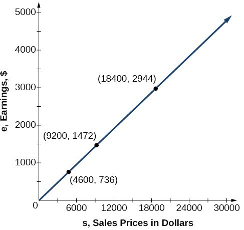
Notice that earnings are a multiple of sales. As sales increase, earnings increase in a predictable way. Double the sales of the vehicle from $4,600 to $9,200, and we double the earnings from $736 to $1,472. As the input increases, the output increases as a multiple of the input. A relationship in which one quantity is a constant multiplied by another quantity is called direct variation. Each variable in this type of relationship varies directly with the other.
The graph below represents the data for Nicole’s potential earnings. We say that earnings vary directly with the sales price of the car. The formula [latex]y=k{x}^{n}[/latex] is used for direct variation. The value [latex]k[/latex] is a nonzero constant greater than zero and is called the constant of variation. In this case, [latex]k=0.16[/latex] and [latex]n=1[/latex].
A General Note: Direct Variation
If [latex]x[/latex] and [latex]y[/latex] are related by an equation of the form
[latex]y=k{x}^{n}[/latex]
then we say that the relationship is direct variation and [latex]y[/latex] varies directly with the [latex]n[/latex]th power of [latex]x[/latex]. In direct variation relationships, there is a nonzero constant ratio [latex]k=\dfrac{y}{{x}^{n}}[/latex], where [latex]k[/latex] is called the constant of variation, which help defines the relationship between the variables.
How To: Given a description of a direct variation problem, solve for an unknown
- Identify the input, [latex]x[/latex], and the output, [latex]y[/latex].
- Determine the constant of variation. You may need to divide [latex]y[/latex] by the specified power of [latex]x[/latex] to determine the constant of variation.
- Use the constant of variation to write an equation for the relationship.
- Substitute known values into the equation to find the unknown.
Example: Writing a Direct Variation Equation
The quantity [latex]y[/latex] varies directly with the cube of [latex]x[/latex]. If [latex]y=25[/latex] when [latex]x=2[/latex], write the equation that represents this relationship. Then, find [latex]y[/latex] when [latex]x[/latex] is 6.
Try It
The quantity [latex]y[/latex] varies directly with the square of [latex]y[/latex]. If [latex]y=24[/latex] when [latex]x=3[/latex], find [latex]y[/latex] when [latex]x[/latex] is 4.
Try It
Watch this video to see a quick lesson about direct variation. You will see more worked examples.
Evaluate Inverse Trigonometric Functions
(also in Module 1, Skills Review for Polar Coordinates)
In order to use inverse trigonometric functions, we need to understand that an inverse trigonometric function “undoes” what the original trigonometric function “does,” as is the case with any other function and its inverse. In other words, the domain of the inverse function is the range of the original function, and vice versa, as summarized below.

For example, if [latex]f(x)=\sin x[/latex], then we would write [latex]f^{-1}(x)={\sin}^{-1}{x}[/latex]. Be aware that [latex]{\sin}^{-1}x[/latex] does not mean [latex]\frac{1}{\sin{x}}[/latex]. The following examples illustrate the inverse trigonometric functions:
- Since [latex]\sin\left(\frac{\pi}{6}\right)=\frac{1}{2}[/latex], then [latex]\frac{\pi}{6}=\sin^{−1}(\frac{1}{2})[/latex].
- Since [latex]\cos(\pi)=−1[/latex], then [latex]\pi=\cos^{−1}(−1)[/latex].
- Since [latex]\tan\left(\frac{\pi}{4}\right)=1[/latex], then [latex]\frac{\pi}{4}=\tan^{−1}(1)[/latex].
A General Note: Relations for Inverse Sine, Cosine, and Tangent Functions
For angles in the interval [latex]\left[−\frac{\pi}{2}\text{, }\frac{\pi}{2}\right][/latex], if [latex]\sin y=x[/latex], then [latex]\sin^{−1}x=y[/latex].
For angles in the interval [0, π], if [latex]\cos y=x[/latex], then [latex]\cos^{−1}x=y[/latex].
For angles in the interval [latex]\left(−\frac{\pi}{2}\text{, }\frac{\pi}{2}\right)[/latex], if [latex]\tan y=x[/latex], then [latex]\tan^{−1}x=y[/latex].
Just as we did with the original trigonometric functions, we can give exact values for the inverse functions when we are using the special angles, specifically [latex]\frac{\pi}{ 6} (30^\circ)\text{, }\frac{\pi}{ 4} (45^\circ),\text{ and } \frac{\pi}{ 3} (60^\circ)[/latex], and their reflections into other quadrants.
How To: Given a “special” input value, evaluate an inverse trigonometric function.
- Find angle x for which the original trigonometric function has an output equal to the given input for the inverse trigonometric function.
- If x is not in the defined range of the inverse, find another angle y that is in the defined range and has the same sine, cosine, or tangent as x, depending on which corresponds to the given inverse function.
Example: Evaluating Inverse Trigonometric Functions for Special Input Values
Evaluate each of the following.
a. [latex]\sin−1\left(\frac{1}{2}\right)[/latex]
b. [latex]\sin−1\left(−\frac{2}{\sqrt{2}}\right)[/latex]
c. [latex]\cos−1\left(−\frac{3}{\sqrt{2}}\right)[/latex]
d. [latex]\tan^{− 1}(1)[/latex]
Try It
Evaluate each of the following.
- [latex]\sin^{−1}(−1)[/latex]
- [latex]\tan^{−1}(−1)[/latex]
- [latex]\cos^{−1}(−1)[/latex]
- [latex]\cos^{−1}(\frac{1}{2})[/latex]
Try It
Note that sometimes you will not be able to find an exact angle measure for a given inverse trigonometric function. Instead, you can use a calculator. First, be sure you put the calculator in the correct mode (degrees or radians). Then, select the inverse trigonometric function of interest along with the corresponding values that go inside the function. Your calculator will then give you the angle measure in degrees (if in degree mode) or in radians (if in radian mode).
Candela Citations
- Calculus Volume 1. Provided by: Lumen Learning. Located at: https://courses.lumenlearning.com/calculus1/. License: CC BY: Attribution
- Calculus Volume 2. Provided by: Lumen Learning. Located at: https://courses.lumenlearning.com/calculus2/. License: CC BY: Attribution
