Learning Outcomes
- Apply basic derivative rules
- Apply the chain rule together with the power and product rule
- Evaluate composite functions
- Apply the Pythagorean identities
- Evaluate trigonometric functions at specific angle measures
In the Line Integrals section, we will learn how to integrate multivariable functions and vector fields over arbitrary curves in a plane or space. In the Conservative Vector Fields section, we will learn about building conservative vector fields and evaluating them using the Fundamental Theorem for Line Integrals. Here we will review how to take derivatives of functions, plug functions into each other, use Pythagorean identities, and evaluate trigonometric functions at specific angle measures.
Basic Derivative Rules
(also in Module 3, Skills Review for Calculus of Vector-Valued Functions)
We first apply the limit definition of the derivative to find the derivative of the constant function, [latex]f(x)=c[/latex]. For this function, both [latex]f(x)=c[/latex] and [latex]f(x+h)=c[/latex], so we obtain the following result:
The rule for differentiating constant functions is called the constant rule. It states that the derivative of a constant function is zero; that is, since a constant function is a horizontal line, the slope, or the rate of change, of a constant function is 0. We restate this rule in the following theorem.
The Constant Rule
Let [latex]c[/latex] be a constant.
If [latex]f(x)=c[/latex], then [latex]f^{\prime}(c)=0[/latex]
Alternatively, we may express this rule as
[latex]\dfrac{d}{dx}(c)=0[/latex]
Example: Applying the Constant Rule
Find the derivative of [latex]f(x)=8[/latex].
Try It
Find the derivative of [latex]g(x)=-3[/latex].
We have shown that
At this point, you might see a pattern beginning to develop for derivatives of the form [latex]\frac{d}{dx}(x^n)[/latex]. We continue our examination of derivative formulas by differentiating power functions of the form [latex]f(x)=x^n[/latex] where [latex]n[/latex] is a positive integer. We develop formulas for derivatives of this type of function in stages, beginning with positive integer powers. Before stating and proving the general rule for derivatives of functions of this form, we take a look at a specific case, [latex]\frac{d}{dx}(x^3)[/latex].
As we shall see, the procedure for finding the derivative of the general form [latex]f(x)=x^n[/latex] is very similar. Although it is often unwise to draw general conclusions from specific examples, we note that when we differentiate [latex]f(x)=x^3[/latex], the power on [latex]x[/latex] becomes the coefficient of [latex]x^2[/latex] in the derivative and the power on [latex]x[/latex] in the derivative decreases by 1. The following theorem states that this power rule holds for all positive integer powers of [latex]x[/latex]. We will eventually extend this result to negative integer powers. Later, we will see that this rule may also be extended first to rational powers of [latex]x[/latex] and then to arbitrary powers of [latex]x[/latex]. Be aware, however, that this rule does not apply to functions in which a constant is raised to a variable power, such as [latex]f(x)=3^x[/latex].
The Power Rule
Let [latex]n[/latex] be a positive integer. If [latex]f(x)=x^n[/latex], then
Alternatively, we may express this rule as
Example: Applying the Power Rule
Find the derivative of the function [latex]f(x)=x^{10}[/latex] by applying the power rule.
Try It
Find the derivative of [latex]f(x)=x^7[/latex].
We find our next differentiation rules by looking at derivatives of sums, differences, and constant multiples of functions. Just as when we work with functions, there are rules that make it easier to find derivatives of functions that we add, subtract, or multiply by a constant. These rules are summarized in the following theorem.
Sum, Difference, and Constant Multiple Rules
Let [latex]f(x)[/latex] and [latex]g(x)[/latex] be differentiable functions and [latex]k[/latex] be a constant. Then each of the following equations holds.
Sum Rule: The derivative of the sum of a function [latex]f[/latex] and a function [latex]g[/latex] is the same as the sum of the derivative of [latex]f[/latex] and the derivative of [latex]g[/latex].
that is,
Difference Rule: The derivative of the difference of a function [latex]f[/latex] and a function [latex]g[/latex] is the same as the difference of the derivative of [latex]f[/latex] and the derivative of [latex]g[/latex].
that is,
Constant Multiple Rule: The derivative of a constant [latex]k[/latex] multiplied by a function [latex]f[/latex] is the same as the constant multiplied by the derivative:
that is,
Example: Applying Basic Derivative Rules
Find the derivative of [latex]f(x)=2x^5+7[/latex].
Try It
Find the derivative of [latex]f(x)=2x^3-6x^2+3[/latex].
The Chain Rule
(also in Module 3, Skills Review for Calculus of Vector-Valued Functions)
The Chain Rule
Let [latex]f[/latex] and [latex]g[/latex] be functions. For all [latex]x[/latex] in the domain of [latex]g[/latex] for which [latex]g[/latex] is differentiable at [latex]x[/latex] and [latex]f[/latex] is differentiable at [latex]g(x)[/latex], the derivative of the composite function
is given by
Alternatively, if [latex]y[/latex] is a function of [latex]u[/latex], and [latex]u[/latex] is a function of [latex]x[/latex], then
Note that we often need to use the chain rule with other rules. For example, to find derivatives of functions of the form [latex]h(x)=(g(x))^n[/latex], we need to use the chain rule combined with the power rule. To do so, we can think of [latex]h(x)=(g(x))^n[/latex] as [latex]f(g(x))[/latex] where [latex]f(x)=x^n[/latex]. Then [latex]f^{\prime}(x)=nx^{n-1}[/latex]. Thus, [latex]f^{\prime}(g(x))=n(g(x))^{n-1}[/latex]. This leads us to the derivative of a power function using the chain rule,
Power Rule for Composition of Functions
For all values of [latex]x[/latex] for which the derivative is defined, if
Then
Example: Using the Chain and Power Rules
Find the derivative of [latex]h(x)=\dfrac{1}{(3x^2+1)^2}[/latex]
Try It
Find the derivative of [latex]h(x)=(2x^3+2x-1)^4[/latex]
Example: Using the Chain and Power Rules with a Trigonometric Function
Find the derivative of [latex]h(x)=\sin^3 x[/latex]
Now that we can combine the chain rule and the power rule, we examine how to combine the chain rule with the other rules we have learned. In particular, we can use it with the formulas for the derivatives of trigonometric functions or with the product rule.
Example: Using the Chain Rule on a Cosine Function
Find the derivative of [latex]h(x)= \cos (5x^2)[/latex].
Example: Using the Chain Rule on Another Trigonometric Function
Find the derivative of [latex]h(x)= \sec (4x^5+2x)[/latex].
Try It
Find the derivative of [latex]h(x)= \sin (7x+2)[/latex].
We now provide a list of derivative formulas that may be obtained by applying the chain rule in conjunction with the formulas for derivatives of trigonometric functions.
Using the Chain Rule with Trigonometric Functions
For all values of [latex]x[/latex] for which the derivative is defined,
[latex]\begin{array}{llll}\frac{d}{dx}(\sin (g(x)))= \cos (g(x))g^{\prime}(x) & & & \frac{d}{dx} \sin u= \cos u\frac{du}{dx} \\ \frac{d}{dx}(\cos (g(x)))=−\sin (g(x))g^{\prime}(x) & & & \frac{d}{dx} \cos u=−\sin u\frac{du}{dx} \\ \frac{d}{dx}(\tan (g(x)))= \sec^2 (g(x))g^{\prime}(x) & & & \frac{d}{dx} \tan u=\sec^2 u\frac{du}{dx} \\ \frac{d}{dx}(\cot (g(x)))=−\csc^2 (g(x))g^{\prime}(x) & & & \frac{d}{dx} \cot u=−\csc^2 u\frac{du}{dx} \\ \frac{d}{dx}(\sec (g(x)))= \sec (g(x)) \tan (g(x))g^{\prime}(x) & & & \frac{d}{dx} \sec u= \sec u \tan u\frac{du}{dx} \\ \frac{d}{dx}(\csc (g(x)))=−\csc (g(x)) \cot (g(x))g^{\prime}(x) & & & \frac{d}{dx} \csc u=−\csc u \cot u\frac{du}{dx} \end{array}[/latex]
Find Composite Functions
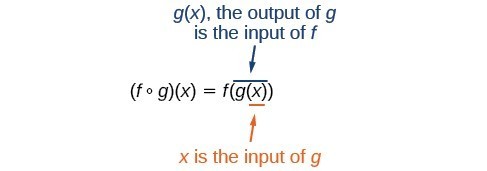
We can create functions by composing them. The process of combining functions so that the output of one function becomes the input of another is known as a composition of functions. The resulting function is known as a composite function. We represent this combination by the following notation:
[latex]\left(f\circ g\right)\left(x\right)=f\left(g\left(x\right)\right)[/latex]
We read the left-hand side as [latex]"f[/latex] composed with [latex]g[/latex] at [latex]x,"[/latex] and the right-hand side as [latex]"f[/latex] of [latex]g[/latex] of [latex]x."[/latex] The two sides of the equation have the same mathematical meaning and are equal. The open circle symbol [latex]\circ[/latex] is called the composition operator. We use this operator mainly when we wish to emphasize the relationship between the functions themselves without referring to any particular input value.
It is also important to understand the order of operations in evaluating a composite function. We follow the usual convention with parentheses by starting with the innermost parentheses first, and then working to the outside. In the equation above, the function [latex]g[/latex] takes the input [latex]x[/latex] first and yields an output [latex]g\left(x\right)[/latex]. Then the function [latex]f[/latex] takes [latex]g\left(x\right)[/latex] as an input and yields an output [latex]f\left(g\left(x\right)\right)[/latex].
In general [latex]f\circ g[/latex] and [latex]g\circ f[/latex] are different functions. In other words in many cases [latex]f\left(g\left(x\right)\right)\ne g\left(f\left(x\right)\right)[/latex] for all [latex]x[/latex].
For example if [latex]f\left(x\right)={x}^{2}[/latex] and [latex]g\left(x\right)=x+2[/latex], then
[latex]\begin{align}f\left(g\left(x\right)\right)&=f\left(x+2\right) \\[2mm] &={\left(x+2\right)}^{2} \\[2mm] &={x}^{2}+4x+4\hfill \end{align}[/latex]
but
[latex]\begin{align}g\left(f\left(x\right)\right)&=g\left({x}^{2}\right) \\[2mm] \text{ }&={x}^{2}+2\hfill \end{align}[/latex]
These expressions are not equal.
Example: Find a CompositE Function
Using the functions provided, find [latex]f\left(g\left(x\right)\right)[/latex] and [latex]g\left(f\left(x\right)\right)[/latex].
[latex]f\left(x\right)=2x+1\\g\left(x\right)=3-x[/latex]
try it
Apply the Pythagorean Identities
Pythagorean identities are equations involving trigonometric functions based on the properties of a right triangle.
| Pythagorean Identities | ||
|---|---|---|
| [latex]{\sin }^{2}\theta +{\cos }^{2}\theta =1[/latex] | [latex]1+{\tan }^{2}\theta ={\sec }^{2}\theta[/latex] | [latex]1+{\cot }^{2}\theta ={\csc }^{2}\theta[/latex] |
- [latex]{\cos }^{2}\theta =1-{\sin }^{2}\theta[/latex]
- [latex]{\sin }^{2}\theta =1 - {\cos }^{2}\theta[/latex]
- [latex]{\tan }^{2}\theta = {\sec }^{2}\theta - 1[/latex]
- [latex]{\sec }^{2}\theta = 1+{\tan }^{2}\theta[/latex] (same as the original identity but sides of the equation are swapped)
Example: Using Pythagorean Identities to Rewrite Expressions
Simplify [latex]\frac{{\sec }^{2}\theta -1}{{\sec }^{2}\theta }[/latex].
Example: Using Pythagorean Identities to Rewrite Expressions
Rewrite the expression [latex]{\sin}\theta {\cos^4}\theta[/latex] using the identity [latex]{\cos }^{2}\theta =1 - {\sin }^{2}\theta[/latex].
.
Try It
Rewrite the expression [latex]{\tan^4}\theta[/latex] using the identity [latex]{\tan }^{2}\theta = {\sec }^{2}\theta - 1[/latex].
Try It
Rewrite the expression [latex]{\sin^2}\theta {\cos}\theta[/latex] using the identity [latex]{\sin }^{2}\theta =1 - {\cos }^{2}\theta[/latex].
Evaluate Trigonometric Functions
Candela Citations
- Calculus Volume 1. Provided by: Lumen Learning. Located at: https://courses.lumenlearning.com/calculus1/. License: CC BY: Attribution
- Calculus Volume 2. Provided by: Lumen Learning. Located at: https://courses.lumenlearning.com/calculus2/. License: CC BY: Attribution

Hint
Use the previous example with [latex]g(x)=2x^3+2x-1[/latex]