Learning Outcomes
- Describe the meaning of the normal and binormal vectors of a curve in space.
We have seen that the derivative [latex]{\bf{r}}'\,(t)[/latex] of a vector-valued function is a tangent vector to the curve defined by [latex]{\bf{r}}\,(t)[/latex], and the unit tangent vector [latex]{\bf{T}}\,(t)[/latex] can be calculated by dividing [latex]{\bf{r}}'\,(t)[/latex] by its magnitude. When studying motion in three dimensions, two other vectors are useful in describing the motion of a particle along a path in space: the principal unit vector and the binomial vector.
Definition
Let [latex]C[/latex] be a three-dimensional smooth curve represented [latex]{\bf{r}}[/latex] over an open interval [latex]I[/latex]. If [latex]{\bf{T}}'\,(t)\neq{0}[/latex], then the principal unit normal vector at [latex]t[/latex] is defined to be
[latex]{\bf{N}}\,(t)=\frac{{\bf{T}}'\,(t)}{\left\Vert{\bf{T}}'\,(t)\right\Vert}[/latex].
The binomial vector at [latex]t[/latex] is defined as
[latex]{\bf{B}}\,(t)={\bf{T}}\,(t)\,\times\,{\bf{N}}\,(t)[/latex],
where [latex]{\bf{T}}(t)[/latex] is the unit tangent vector.
Note that, by definition, the binormal vector is orthogonal to both the unit tangent vector and the normal vector. Furthermore, [latex]{\bf{B}}\,(t)[/latex] is always a unit vector. This cam be shown using the formula for the magnitude of a cross product
[latex]\left\Vert{\bf{B}}\,(t)\right\Vert=\left\Vert{\bf{T}}\,(t)\,\times\,{\bf{N}}\,(t)\right\Vert=\left\Vert{\bf{T}}\,(t)\right\Vert\,\left\Vert{\bf{N}}\,(t)\right\Vert\sin{\theta},[/latex]
where [latex]\theta[/latex] is the angle between [latex]{\bf{T}}\,(t)[/latex] and [latex]{\bf{N}}\,(t)[/latex]. Since [latex]{\bf{N}}\,(t)[/latex] is the derivative of a unit vector, property 7 of the derivative of a vector-valued function tells us that [latex]{\bf{T}}(t)[/latex] and [latex]{\bf{N}}(t)[/latex] are orthogonal to each other, so [latex]\theta=\pi/2[/latex]. Furthermore, they are both unit vectors, so their magnitude is [latex]1[/latex]. Therefore, [latex]\left\Vert{\bf{T}}\,(t)\right\Vert\,\left\Vert{\bf{N}}\,(t)\right\Vert\sin{\theta}=(1)(1)\sin{(\pi/2)}=1[/latex] and [latex]{\bf{B}}\,(t)[/latex] is a unit vector.
The principal unit normal vector can be challenging to calculate because the unit tangent vector involves a quotient, and this quotient often has a square root in the denominator. In the three-dimensional case, finding the cross product of the unit tangent vector and the unit normal vector can be even more cumbersome. Fortunately, we have alternative formulas for finding these two vectors, and they are presented in Motion in Space.
Example: finding the principal unit normal vector and binormal vector
For each of the following vector-valued functions, find the principal unit normal vector. Then, if possible, find the binormal vector.
-
Show Solution
- This function describes a circle.

Figure 1.
To find the principal unit normal vector, we first must find the unit tangent vector [latex]{\bf{T}}\,(t)[/latex]:
[latex]\begin{array}{ccc}\hfill {{\bf{T}}\,(t)} &=\hfill&{\frac{{\bf{r}}'\,(t)}{\left\Vert{\bf{r}}'\,(t)\right\Vert}}\hfill \\ \hfill & =\hfill & {\frac{-4\sin{t{\bf{i}}}-4\cos{t{\bf{j}}}}{\sqrt{(-4\sin{t})^{2}+(-4\cos{t})^{2}}}} \hfill \\ \hfill & =\hfill & {\frac{-4\sin{t{\bf{i}}}-4\cos{t{\bf{j}}}}{\sqrt{16\sin{^{2}t}+16\cos{^{2}t}}}}\hfill \\ \hfill & =\hfill & {\frac{-4\sin{t{\bf{i}}}-4\cos{t{\bf{j}}}}{\sqrt{16(\sin{^{2}t}+\cos{^{2}t})}}}\hfill \\ \hfill & =\hfill & {\frac{-4\sin{t{\bf{i}}}-4\cos{t{\bf{j}}}}{4}}\hfill \\ \hfill & =\hfill & {-\sin{t{\bf{i}}}-\cos{t{\bf{j}}}.}\hfill \\ \hfill \end{array}[/latex]
Next, we use the first equation from the definition
[latex]\begin{array}{ccc}\hfill {{\bf{N}}\,(t)} &=\hfill&{\frac{{\bf{T}}'\,(t)}{\left\Vert{\bf{T}}'\,(t)\right\Vert}}\hfill \\ \hfill & =\hfill & {\frac{-\cos{t{\bf{i}}}+\sin{t{\bf{j}}}}{\sqrt{(-\cos{t})^{2}+(\sin{t})^{2}}}} \hfill \\ \hfill & =\hfill & {\frac{-\cos{t{\bf{i}}}+\sin{t{\bf{j}}}}{\sqrt{\cos{^{2}t}+\sin{^{2}t}}}}\hfill \\ \hfill & =\hfill & {-\cos{t{\bf{i}}}+\sin{t{\bf{j}}}}\hfill \\ \hfill \end{array}[/latex].
Notice that the unit tangent vector and the principal unit normal vector are orthogonal to each other for all rules of [latex]t[/latex]:
[latex]\begin{array}{ccc}\hfill {{\bf{T}}\,(t)\cdot{\bf{N}}\,(t)} &=\hfill&{\langle{-}\sin{t},-\cos{t}\rangle\cdot\langle{-}\cos{t},\sin{t}\rangle}\hfill \\ \hfill & =\hfill & {\sin{t}\cos{t}-\cos{t}\sin{t}} \hfill \\ \hfill & =\hfill & {0.}\hfill \\ \hfill \end{array}[/latex]
Furthermore, the principal unit normal vector points toward the center of the circle from every point on the circle. Since [latex]{\bf{r}}\,(t)[/latex] defines a curve in tow dimensions, we cannot calculate the binormal vector
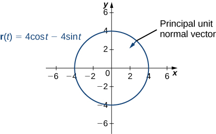
Figure 2.
- This function looks like this:

Figure 3.
To find the principal unit normal vector, we first find the unit tangent vector [latex]{\bf{T}}\,(t)[/latex]:
[latex]\begin{array}{ccc}\hfill {{\bf{T}}\,(t)} &=\hfill & {\frac{{\bf{r}}'\,(t)}{\left\Vert{\bf{r}}'\,(t)\right\Vert}}\hfill \\ \hfill & =\hfill & {\frac{6\,{\bf{i}}+10t\,{\bf{j}}-8\,{\bf{k}}}{\sqrt{6^{2}+(10t)^{2}+(-8)^{2}}}} \hfill \\ \hfill & =\hfill & {\frac{6\,{\bf{i}}+10t\,{\bf{j}}-8\,{\bf{k}}}{\sqrt{36+100t^{2}+64}}}\hfill \\ \hfill & =\hfill & {\frac{6\,{\bf{i}}+10t\,{\bf{j}}-8\,{\bf{k}}}{\sqrt{100(t^{2}+1)}}}\hfill \\ \hfill & =\hfill & {\frac{3\,{\bf{i}}+5t\,{\bf{j}}-4\,{\bf{k}}}{5\,\sqrt{t^{2}+1}}}\hfill \\ \hfill & =\hfill & {\frac{3}{5}\,(t^{2}+1)^{-1/2}{\bf{i}}+t\,(t^{2}+1)^{-1/2}{\bf{j}}-\frac{4}{5}\,(t^{2}+1)^{-1/2}{\bf{k}}.}\hfill \\ \hfill\end{array}[/latex].
Next, we calculate [latex]{\bf{T}}'\,(t)[/latex] and [latex]\left\Vert{\bf{T}}'\,(t)\right\Vert[/latex]:
[latex]\begin{array}{ccc}\hfill {{\bf{T}}\,(t)} &=\hfill & {\frac{3}{5}\,(-\frac{1}{2})\,(t^{2}+1)^{-3/2}(2t)\,{\bf{i}}+\big((t^{2}+1)^{-1/2}-t\,(\frac{1}{2})\,(t^{2}+1)^{-3/2}(2t)\big)\,{\bf{j}}-\frac{4}{5}\,(-\frac{1}{2})\,(t^{2}+1)^{-3/2}(2t)\,{\bf{k}}}\hfill \\ \hfill & =\hfill & {-\frac{3t}{5(t^{2}+1)^{3/2}}\,{\bf{i}}+\frac{1}{(t^{2}+1)^{3/2}}\,{\bf{j}}+\frac{4}{5(t^{2}+1)^{3/2}}\,{\bf{k}}} \hfill \\ \hfill {\left\Vert{\bf{T}}'\,(t)\right\Vert}& =\hfill & {\sqrt{\bigg(-\frac{3t}{5(t^{2}+1)^{3/2}}\bigg)^{2}+\bigg(-\frac{1}{(t^{2}+1)^{3/2}}\bigg)^{2}+\bigg(\frac{4t}{5(t^{2}+1)^{3/2}}\bigg)^{2}}}\hfill \\ \hfill & =\hfill & {\sqrt{\frac{9t^{2}}{25(t^{2}+1)^{3}}+\frac{1}{(t^{2}+1)^{3}}+\frac{16t^{2}}{25(t^{2}+1)^{3}}}}\hfill \\ \hfill & =\hfill & {\sqrt{\frac{25t^{2}+25}{25(t^{2}+1)^{3}}}}\hfill \\ \hfill & =\hfill & {\sqrt{\frac{1}{(t^{2}+1)^{2}}}}\hfill \\ \hfill & =\hfill & {\frac{1}{t^{2}+1}.}\hfill \\ \hfill\end{array}[/latex]
Therefore, according to the second equation from the above definition:
[latex]\begin{array}{ccc}\hfill {{\bf{N}}\,(t)} &=\hfill & {\frac{{\bf{T}}'\,(t)}{\left\Vert{\bf{T}}'\,(t)\right\Vert}}\hfill \\ \hfill & =\hfill & {\bigg(-\frac{3t}{5(t^{2}+1)^{3/2}}{\bf{i}}+\frac{1}{(t^{2}+1)^{3/2}}{\bf{j}}+\frac{4t}{5(t^{2}+1)^{3/2}}{\bf{k}}\bigg)(t^{2}+1)} \hfill \\ \hfill & =\hfill & {-\frac{3t}{5(t^{2}+1)^{1/2}}{\bf{i}}+\frac{1}{(t^{2}+1)^{1/2}}{\bf{j}}+\frac{4t}{5(t^{2}+1)^{1/2}}{\bf{k}}}\hfill \\ \hfill & =\hfill & {-\frac{3t\,{\bf{i}}-5\,{\bf{j}}-4t\,{\bf{k}}}{5\sqrt{t^{2}+1}}}\hfill \\ \hfill\end{array}[/latex]
Once again, the unit tangent vector and the principal unit normal vector are orthogonal to each other for all values of [latex]t[/latex]:
[latex]\begin{array}{ccc}\hfill {{\bf{T}}\,(t)\cdot{\bf{N}}\,(t)} &=\hfill & {\bigg(\frac{3\,{\bf{i}}+5t\,{\bf{j}}-4\,{\bf{k}}}{5\sqrt{t^{2}+1}}\bigg)\cdot\bigg(-\frac{3t\,{\bf{i}}-5\,{\bf{j}}-4t\,{\bf{k}}}{5\sqrt{t^{2}+1}}\bigg)}\hfill \\ \hfill & =\hfill & {\frac{3(-3)-5t(-5)-4(4t)}{5\sqrt{t^{2}+1}}} \hfill \\ \hfill & =\hfill & {\frac{-9t+25t-16t}{5\sqrt{t^{2}+1}}}\hfill \\ \hfill & =\hfill & {0.}\hfill \\ \hfill\end{array}[/latex]
Last, since [latex]{\bf{r}}\,(t)[/latex] represents a three-dimensional curve, we can calculate the binormal vector using the first equation from the above definition:
[latex]\begin{array}{ccc}\hfill {{\bf{B}}\,(t)} &=\hfill & {{\bf{T}}\,(t)\,\times\,{\bf{N}}\,(t)}\hfill \\ \hfill & =\hfill & {\begin{vmatrix}{\bf{i}}&{\bf{j}}&{\bf{k}}\\\frac{3}{5\sqrt{t^{2}+1}}&+\frac{5t}{5\sqrt{t^{2}+1}}&-\frac{4}{5\sqrt{t^{2}+1}}\\ -\frac{3t}{5\sqrt{t^{2}+1}}&+\frac{5}{5\sqrt{t^{2}+1}}&\frac{4t}{5\sqrt{t^{2}+1}}\end{vmatrix}} \hfill \\ \hfill & =\hfill & {\bigg(\Big(+\frac{5t}{5\sqrt{t^{2}+1}}\Big)\Big(\frac{4t}{5\sqrt{t^{2}+1}}\Big)-\Big(-\frac{4}{5\sqrt{t^{2}+1}}\Big)\Big(-\frac{5}{5\sqrt{t^{2}+1}}\Big)\bigg)\,{\bf{i}} \\ +\bigg(\Big(\frac{3}{5\sqrt{t^{2}+1}}\Big)\Big(\frac{4t}{5\sqrt{t^{2}+1}}\Big)-\Big(-\frac{4}{5\sqrt{t^{2}+1}}\Big)\Big(-\frac{3t}{5\sqrt{t^{2}+1}}\Big)\bigg)\,{\bf{j}} \\ +\bigg(\Big(\frac{3}{5\sqrt{t^{2}+1}}\Big)\Big(+\frac{5}{5\sqrt{t^{2}+1}}\Big)-\Big(+\frac{5t}{5\sqrt{t^{2}+1}}\Big)\Big(-\frac{3t}{5\sqrt{t^{2}+1}}\Big)\bigg){\bf{k}}}\hfill \\ \hfill & =\hfill & {\Big(\frac{20t^{2}+20}{25(t^{2}+1)}\Big)\,{\bf{i}}+\Big(\frac{-15-15t^{2}}{25(t^{2}+1)}\Big)\,{\bf{k}}}\hfill \\ \hfill & =\hfill & {20\,\Big(\frac{t^{2}+1}{25(t^{2}+1)}\Big)\,{\bf{i}}-15\,\Big(\frac{t^{2}+1}{25(t^{2}+1)}\Big)\,{\bf{k}}}\hfill \\ \hfill & =\hfill & {\frac{4}{5}\,{\bf{i}}-\frac{3}{5}\,{\bf{k}}.}\hfill \\ \hfill\end{array}[/latex]
try it
Find the unit normal vector for the vector-valued function [latex]{\bf{r}}\,(t)=(t^{2}-3)\,{\bf{I}}+(4t+1)\,{\bf{j}}[/latex] and evaluate it at [latex]t=2[/latex].
Show Solution
[latex]\kappa=\frac{6}{101^{3/2}}\approx{0.0059}[/latex]
For any smooth curve in three dimensions that is defined by a vector-valued function, we now have formulas for the unit tangent vector [latex]{\bf{T}}[/latex], the unit normal vector [latex]{\bf{N}}[/latex], and the binormal vector [latex]\bf{B}[/latex]. The unit normal vector and the binormal vector form a plane that is perpendicular to the curve at any point on the curve, called the normal plane. In addition, these three vectors form a frame of reference in three-dimensional space called the Frenet frame of reference (also called the TNB frame) (Figure 7). Lat, the plane determined by the vectors [latex]\bf{T}[/latex] and [latex]\bf{N}[/latex] forms the osculating plane of [latex]C[/latex] at any point [latex]P[/latex] on the curve.

Figure 4. This figure depicts a Frenet frame of reference. At every point [latex]P[/latex] on a three-dimensional curve, the unit tangent, unit normal, and binormal vectors form a three-dimensional frame of reference.
Suppose we form a circle in the osculating plane of [latex]C[/latex] at point [latex]P[/latex] on the curve. Assume that the circle has the same curvature as the curve does at point [latex]P[/latex] and let the circle have radius [latex]r[/latex]. Then, the curvature of the circle is given by [latex]1/r[/latex]. We call [latex]r[/latex] the radius of curvature of the curve, and it is equal to the reciprocal of the curvature. If this circle lies on the concave side of the curve and is tangent to the curve at point [latex]P[/latex], then this circle is called the osculating circle of [latex]C[/latex] at [latex]P[/latex], as shown in the following figure.

Figure 5. In this osculating circle, the circle is tangent to curve [latex]C[/latex] at point [latex]P[/latex] and shares the same curvature.
Interactive
For more information on osculating circles, see this demonstration on curvature and torsion, this article on osculating circles, and this discussion of Serret formulas.
To find the equation of an osculating circle in two dimensions, we need find only the center and radius of the circle.
Example: finding the Equation of an Osculating Circle
Find the equation of the osculating circle of the helix defined by the function [latex]y=x^{3}-3x+1[/latex] at [latex]x=1[/latex].
Show Solution
Figure 9 shows the graph of [latex]y=x^{3}-3x+1[/latex].

Figure 6. We want to find the osculating circle of this graph at the point where [latex]t=1[/latex].
First, let’s calculate the curvature at [latex]x=1[/latex]:
[latex]\LARGE{\kappa=\frac{|f''\,(x)|}{(1+[f'\,(x)]^{2})^{3/2}}=\frac{|6x|}{(1+[3x^{2}-3]^{2})^{3/2}}}.[/latex]
This gives [latex]\kappa=6[/latex]. Therefore, the radius of the osculating circle is given by [latex]R=\frac{1}{\kappa}=\frac{1}{6}[/latex]. Next, we then calculate the coordinates of the center of the circle. When [latex]x=1[/latex], the slope of the tangent line is zero. Therefore, the center of the osculating circle is directly above the point on the graph with coordinates [latex](1,\ -1)[/latex]. The center is located at [latex](1,\ -\frac{5}{6})[/latex]. The formula for a circle with radius [latex]r[/latex] and center [latex](h,\ k)[/latex] is given by [latex](x-h)^{2}+(y-k)^{2}=r^{2}[/latex]. Therefore, the equation of the osculating circle is [latex](x-1)^{2}+(y+\frac{5}{6})^{2}=\frac{1}{36}[/latex]. The graph and its osculating circle appears in the following graph.

Figure 8. The osculating circle has radius [latex]R=\frac{1}{6}[/latex]
try it
Find the equation of the osculating circle of the curve defined by the vector-valued function [latex]y=2x^{2}-4x+5[/latex] at [latex]x=1[/latex].
Show Solution
[latex]\kappa=\frac{4}{[1+(4x-4)^{2}]^{3/2}}[/latex] At the point [latex]x=1[/latex], the curvature is equal to [latex]4[/latex]. Therefore, the radius of the osculating circle is [latex]\frac{1}{4}[/latex]. A graph of this functions appears next:

Figure 9.
The vertex of this parabola is located at the point [latex](1,\ 3)[/latex]. Furthermore, the center of the osculating circle is directly above the vertex. Therefore, the coordinates of the center are [latex](1,\ \frac{13}{4})[/latex]. The equation of the osculating circle is [latex](x-1)^{2}+(y-\frac{13}{4})^{2}=\frac{1}{16}[/latex].
[latex]{\bf{v}}\,(t)={\bf{r}}'\,(t)=(2t-3)\,{\bf{i}}+2\,{\bf{j}}+{\bf{k}}[/latex]
Watch the following video to see the worked solution to the above Try It
Candela Citations
CC licensed content, Original
CC licensed content, Shared previously
