Introduction

What you’ll learn to do: Recognize scenarios that can be modeled by logistic growth

In a confined environment the growth rate of a population may not remain constant. In a lake, for example, there is some maximum sustainable population of fish, also called a carrying capacity. In this section, we will develop a model that contains a carrying capacity term, and use it to predict growth under constraints.  Because resources are typically limited in systems, these types of models are much more common than linear or exponential growth.

The famous Mandelbrot set, a fractal whose growth is constrained.

Logistic Growth

Limits on Exponential Growth

In our basic exponential growth scenario, there was no limit to the growth of the output.  That is, as the input got larger the output grew without bound.  In a confined environment, however, the growth rate may not remain constant. Considering our example in the previous section of fish population in a lake, there would be some maximum sustainable population of fish.  We call this number the carrying capacity.

For our fish, the carrying capacity is the largest population that the resources in the lake can sustain. If the population in the lake is far below the carrying capacity, then we would expect the population to grow essentially exponentially. However, as the population approaches the carrying capacity, there will be a scarcity of food and space available, and the growth rate will decrease. If the population exceeds the carrying capacity, there won’t be enough resources to sustain all the fish and there will be a negative growth rate, causing the population to decrease back to the carrying capacity.

Logistic Growth

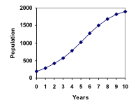
If a population with initial value P₀ is growing in a constrained environment with carrying capacity K, and absent constraint would grow exponentially with growth rate r, then the population behavior can be described by the logistic growth model.  We will not discuss the formula for this model, but rather the shape of the graph made by this model.  Such a model would start out looking like the exponential growth model with initial value P₀ and growth rate r.  But it does not continue to grow without bound.  Rather, it begins to flatten out and approach the carrying capacity as shown in the graph below:

 

So let’s take another look at our fish population example.  The initial fish population in the lake was 1000 fish and 10% of the fish have surviving offspring each year.  If we adjust the model to include a carrying capacity of 6000 fish, then the model looks like this:

Notice that the graph looks a lot like the exponential model we created in the last section for fish population until about 15 years out.  Then the curve begins to flatten.

Examples

A forest is currently home to a population of 200 rabbits. The forest is estimated to be able to sustain a population of 2000 rabbits. Absent any restrictions, the rabbit population would grow by 50% per year. Would you expect this scenario to be modeled by linear, exponential, or logistic growth.

Show Solution

Since the rabbit population grow by about 50% per year (percent change), we would expect this scenario to be modeled, at least initially, by exponential growth.  However, since there are factors limiting the forest to be able to sustain a population of approximately 2000 rabbits, then we would expect a logistic growth model to give the best fit for this scenario.

Indeed, such a model gives the following graph. [Note: you will not be required to create a formula for the logistic growth model.] Notice that the population starts to increase faster and the graph curves upwards during the first few years, like exponential growth, but then the growth slows down as the population approaches the carrying capacity.