Growth models can help us to understand the world around us. In this module, we have learned to describe and compare growth by understanding a little bit about different types of growth.
We saw that linear growth is characterized by having a constant rate of change. When something is increasing linearly, it increases by the same amount every year (or every month, every day, etc.). Because of this, graphs which model linear growth are straight lines.
Exponential growth is similar, except that instead of increasing by the same amount every year, quantities increase by the same percent each year. The constant percent change is called the growth rate. What this means for exponential growth, is that every year the increase will be by a bigger amount than it was the previous year (in the next module this will have an importance consequence, called compounding). This implies that graphs which model exponential growth look like:

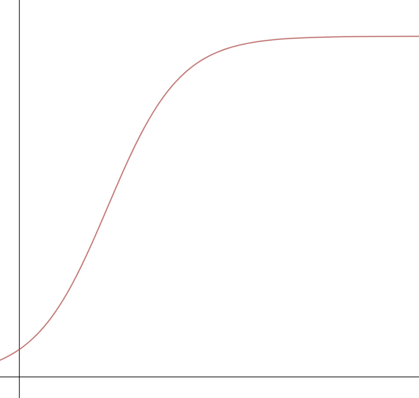
The third type of growth that we explored was logistic growth. One important idea behind logistic growth is that there is often a `ceiling’ which caps the amount of growth that can occur. For example, there are only so many fish that a particular ecosystem can support. The maximum sustainable population is called the carrying capacity. Graphs of logistic models generally appear exponential in the beginning and then flatten over time as shown in the following graph:
We also used growth models to make predictions. For linear growth, we used the explicit formula:
\[ P_n = P_0 +dn,\]
where [latex]P_n[/latex] is the amount present after [latex]n[/latex] years/days/months, [latex]P_0[/latex] is the initial amount, and [latex]d[/latex] is the constant rate of change.
For exponential growth, our explicit formula is:
\[P_n = P_0 \left(1+r\right)^n,\]
where [latex]r[/latex] is the growth rate (written as a decimal).
(For those who are curious, there is also an explicit formula for logistic growth. Understanding where the formula comes from typically involves calculus though, so we won’t use it in this class.)
When making predictions, it is important to keep in mind that some models may exhibit linear or exponential growth in the short-run but the models might change in the future. Because of this we should always be careful whenever we extrapolate (i.e.: extend our model or graph by inferring unknown values from trends in the known data).

Candela Citations
- Putting It Together: Growth Models. Authored by: Lumen Learning. License: CC BY: Attribution
- Photography model on beach. Located at: https://www.pexels.com/photo/blur-camera-capture-close-up-175655. License: CC0: No Rights Reserved