Figure 1. Devastation of January 2010 earthquake in Haiti.

In 2010, a major earthquake struck Haiti, destroying or damaging over 285,000 homes.^[1] One year later, another, stronger earthquake devastated Honshu, Japan, destroying or damaging over 332,000 buildings,^[2] like those shown in the picture above. Even though both caused substantial damage, the earthquake in 2011 was 100 times stronger than the earthquake in Haiti. How do we know? The magnitudes of earthquakes are measured on a scale known as the Richter Scale. The Haitian earthquake registered a 7.0 on the Richter Scale^[3] whereas the Japanese earthquake registered a 9.0.^[4]

The Richter Scale is a base-ten logarithmic scale. In other words, an earthquake of magnitude 8 is not twice as great as an earthquake of magnitude 4. It is [latex]{10}^{8 - 4}={10}^{4}=10,000[/latex] times as great! In this lesson, we will investigate the nature of the Richter Scale and the base-ten function upon which it depends.

Convert from logarithmic to exponential form

In order to analyze the magnitude of earthquakes or compare the magnitudes of two different earthquakes, we need to be able to convert between logarithmic and exponential form. For example, suppose the amount of energy released from one earthquake were 500 times greater than the amount of energy released from another. We want to calculate the difference in magnitude. The equation that represents this problem is [latex]{10}^{x}=500[/latex], where x represents the difference in magnitudes on the Richter Scale. How would we solve for x?

We have not yet learned a method for solving exponential equations. None of the algebraic tools discussed so far is sufficient to solve [latex]{10}^{x}=500[/latex]. We know that [latex]{10}^{2}=100[/latex] and [latex]{10}^{3}=1000[/latex], so it is clear that x must be some value between 2 and 3, since [latex]y={10}^{x}[/latex] is increasing. We can examine a graph to better estimate the solution.

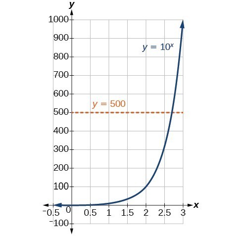
Figure 2

Estimating from a graph, however, is imprecise. To find an algebraic solution, we must introduce a new function. Observe that the graph above passes the horizontal line test. The exponential function [latex]y={b}^{x}[/latex] is one-to-one, so its inverse, [latex]x={b}^{y}[/latex] is also a function. As is the case with all inverse functions, we simply interchange x and y and solve for y to find the inverse function. To represent y as a function of x, we use a logarithmic function of the form [latex]y={\mathrm{log}}_{b}\left(x\right)[/latex]. The base b logarithm of a number is the exponent by which we must raise b to get that number.

We read a logarithmic expression as, “The logarithm with base b of x is equal to y,” or, simplified, “log base b of x is y.” We can also say, “b raised to the power of y is x,” because logs are exponents. For example, the base 2 logarithm of 32 is 5, because 5 is the exponent we must apply to 2 to get 32. Since [latex]{2}^{5}=32[/latex], we can write [latex]{\mathrm{log}}_{2}32=5[/latex]. We read this as “log base 2 of 32 is 5.”

We can express the relationship between logarithmic form and its corresponding exponential form as follows:

[latex]{\mathrm{log}}_{b}\left(x\right)=y\Leftrightarrow {b}^{y}=x,\text{}b>0,b\ne 1[/latex]

Note that the base b is always positive.

Because logarithm is a function, it is most correctly written as [latex]{\mathrm{log}}_{b}\left(x\right)[/latex], using parentheses to denote function evaluation, just as we would with [latex]f\left(x\right)[/latex]. However, when the input is a single variable or number, it is common to see the parentheses dropped and the expression written without parentheses, as [latex]{\mathrm{log}}_{b}x[/latex]. Note that many calculators require parentheses around the x.

We can illustrate the notation of logarithms as follows:

Notice that, comparing the logarithm function and the exponential function, the input and the output are switched. This means [latex]y={\mathrm{log}}_{b}\left(x\right)[/latex] and [latex]y={b}^{x}[/latex] are inverse functions.

A General Note: Definition of the Logarithmic Function

A logarithm base b of a positive number x satisfies the following definition.

For [latex]x>0,b>0,b\ne 1[/latex],

[latex]y={\mathrm{log}}_{b}\left(x\right)\text{ is equivalent to }{b}^{y}=x[/latex]

where,

• we read [latex]{\mathrm{log}}_{b}\left(x\right)[/latex] as, “the logarithm with base b of x” or the “log base b of x.”
• the logarithm y is the exponent to which b must be raised to get x.

Also, since the logarithmic and exponential functions switch the x and y values, the domain and range of the exponential function are interchanged for the logarithmic function. Therefore,

• the domain of the logarithm function with base [latex]b \text{ is} \left(0,\infty \right)[/latex].
• the range of the logarithm function with base [latex]b \text{ is} \left(-\infty ,\infty \right)[/latex].

Q & A

Can we take the logarithm of a negative number?

No. Because the base of an exponential function is always positive, no power of that base can ever be negative. We can never take the logarithm of a negative number. Also, we cannot take the logarithm of zero. Calculators may output a log of a negative number when in complex mode, but the log of a negative number is not a real number.

How To: Given an equation in logarithmic form [latex]{\mathrm{log}}_{b}\left(x\right)=y[/latex], convert it to exponential form.

1. Examine the equation [latex]y={\mathrm{log}}_{b}x[/latex] and identify b, y, and x.
2. Rewrite [latex]{\mathrm{log}}_{b}x=y[/latex] as [latex]{b}^{y}=x[/latex].

Example 1: Converting from Logarithmic Form to Exponential Form

Write the following logarithmic equations in exponential form.

1. [latex]{\mathrm{log}}_{6}\left(\sqrt{6}\right)=\frac{1}{2}[/latex]
2. [latex]{\mathrm{log}}_{3}\left(9\right)=2[/latex]

Show Solution

First, identify the values of b, y, and x. Then, write the equation in the form [latex]{b}^{y}=x[/latex].

1. [latex]{\mathrm{log}}_{6}\left(\sqrt{6}\right)=\frac{1}{2}[/latex]

   Here, [latex]b=6,y=\frac{1}{2},\text{and } x=\sqrt{6}[/latex]. Therefore, the equation [latex]{\mathrm{log}}_{6}\left(\sqrt{6}\right)=\frac{1}{2}[/latex] is equivalent to [latex]{6}^{\frac{1}{2}}=\sqrt{6}[/latex].

2. [latex]{\mathrm{log}}_{3}\left(9\right)=2[/latex]

   Here, b = 3, y = 2, and x = 9. Therefore, the equation [latex]{\mathrm{log}}_{3}\left(9\right)=2[/latex] is equivalent to [latex]{3}^{2}=9[/latex].

Try It

Write the following logarithmic equations in exponential form.

a. [latex]{\mathrm{log}}_{10}\left(1,000,000\right)=6[/latex]

b. [latex]{\mathrm{log}}_{5}\left(25\right)=2[/latex]

Show Solution

a. [latex]{\mathrm{log}}_{10}\left(1,000,000\right)=6[/latex] is equivalent to [latex]{10}^{6}=1,000,000[/latex]
b. [latex]{\mathrm{log}}_{5}\left(25\right)=2[/latex] is equivalent to [latex]{5}^{2}=25[/latex]

Try It

 Convert from exponential to logarithmic form

To convert from exponents to logarithms, we follow the same steps in reverse. We identify the base b, exponent x, and output y. Then we write [latex]x={\mathrm{log}}_{b}\left(y\right)[/latex].

 Evaluate logarithms

Knowing the squares, cubes, and roots of numbers allows us to evaluate many logarithms mentally. For example, consider [latex]{\mathrm{log}}_{2}8[/latex]. We ask, “To what exponent must 2 be raised in order to get 8?” Because we already know [latex]{2}^{3}=8[/latex], it follows that [latex]{\mathrm{log}}_{2}8=3[/latex].

Now consider solving [latex]{\mathrm{log}}_{7}49[/latex] and [latex]{\mathrm{log}}_{3}27[/latex] mentally.

• We ask, “To what exponent must 7 be raised in order to get 49?” We know [latex]{7}^{2}=49[/latex]. Therefore, [latex]{\mathrm{log}}_{7}49=2[/latex]
• We ask, “To what exponent must 3 be raised in order to get 27?” We know [latex]{3}^{3}=27[/latex]. Therefore, [latex]{\mathrm{log}}_{3}27=3[/latex]

Even some seemingly more complicated logarithms can be evaluated without a calculator. For example, let’s evaluate [latex]{\mathrm{log}}_{\frac{2}{3}}\frac{4}{9}[/latex] mentally.

• We ask, “To what exponent must [latex]\frac{2}{3}[/latex] be raised in order to get [latex]\frac{4}{9}[/latex]? ” We know [latex]{2}^{2}=4[/latex] and [latex]{3}^{2}=9[/latex], so [latex]{\left(\frac{2}{3}\right)}^{2}=\frac{4}{9}[/latex]. Therefore, [latex]{\mathrm{log}}_{\frac{2}{3}}\left(\frac{4}{9}\right)=2[/latex].

How To: Given a logarithm of the form [latex]y={\mathrm{log}}_{b}\left(x\right)[/latex], evaluate it mentally.

1. Rewrite the argument x as a power of b: [latex]{b}^{y}=x[/latex].
2. Use previous knowledge of powers of b identify y by asking, “To what exponent should b be raised in order to get x?”

Example 3: Solving Logarithms Mentally

Solve [latex]y={\mathrm{log}}_{4}\left(64\right)[/latex] without using a calculator.

Show Solution

First we rewrite the logarithm in exponential form: [latex]{4}^{y}=64[/latex]. Next, we ask, “To what exponent must 4 be raised in order to get 64?”

We know

[latex]{4}^{3}=64[/latex]

Therefore,

[latex]\mathrm{log}{}_{4}\left(64\right)=3[/latex]

Try It

Solve [latex]y={\mathrm{log}}_{121}\left(11\right)[/latex] without using a calculator.

Show Solution

[latex]{\mathrm{log}}_{121}\left(11\right)=\frac{1}{2}[/latex] (recalling that [latex]\sqrt{121}={\left(121\right)}^{\frac{1}{2}}=11[/latex])

Example 4: Evaluating the Logarithm of a Reciprocal

Evaluate [latex]y={\mathrm{log}}_{3}\left(\frac{1}{27}\right)[/latex] without using a calculator.

Show Solution

First we rewrite the logarithm in exponential form: [latex]{3}^{y}=\frac{1}{27}[/latex]. Next, we ask, “To what exponent must 3 be raised in order to get [latex]\frac{1}{27}[/latex]“?

We know [latex]{3}^{3}=27[/latex], but what must we do to get the reciprocal, [latex]\frac{1}{27}[/latex]? Recall from working with exponents that [latex]{b}^{-a}=\frac{1}{{b}^{a}}[/latex]. We use this information to write

[latex]\begin{align}{3}^{-3}&=\frac{1}{{3}^{3}} \\ &=\frac{1}{27} \end{align}[/latex]

Therefore, [latex]{\mathrm{log}}_{3}\left(\frac{1}{27}\right)=-3[/latex].

Try It

Evaluate [latex]y={\mathrm{log}}_{2}\left(\frac{1}{32}\right)[/latex] without using a calculator.

Show Solution

[latex]{\mathrm{log}}_{2}\left(\frac{1}{32}\right)=-5[/latex]

Try It

 Use common logarithms

The most frequently used base for logarithms is e. Base e logarithms are important in calculus and some scientific applications; they are called natural logarithms. The base e logarithm, [latex]{\mathrm{log}}_{e}\left(x\right)[/latex], has its own notation, [latex]\mathrm{ln}\left(x\right)[/latex].

Most values of [latex]\mathrm{ln}\left(x\right)[/latex] can be found only using a calculator. The major exception is that, because the logarithm of 1 is always 0 in any base, [latex]\mathrm{ln}1=0[/latex]. For other natural logarithms, we can use the [latex]\mathrm{ln}[/latex] key that can be found on most scientific calculators. We can also find the natural logarithm of any power of e using the inverse property of logarithms.

A General Note: Definition of the Natural Logarithm

A natural logarithm is a logarithm with base e. We write [latex]{\mathrm{log}}_{e}\left(x\right)[/latex] simply as [latex]\mathrm{ln}\left(x\right)[/latex]. The natural logarithm of a positive number x satisfies the following definition.

For [latex]x>0[/latex],

[latex]y=\mathrm{ln}\left(x\right)\text{ is equivalent to }{e}^{y}=x[/latex]

We read [latex]\mathrm{ln}\left(x\right)[/latex] as, “the logarithm with base e of x” or “the natural logarithm of x.”

The logarithm y is the exponent to which e must be raised to get x.

Since the functions [latex]y=e{}^{x}[/latex] and [latex]y=\mathrm{ln}\left(x\right)[/latex] are inverse functions, [latex]\mathrm{ln}\left({e}^{x}\right)=x[/latex] for all x and [latex]e{}^{\mathrm{ln}\left(x\right)}=x[/latex] for x > 0.

How To: Given a natural logarithm with the form [latex]y=\mathrm{ln}\left(x\right)[/latex], evaluate it using a calculator.

1. Press [LN].
2. Enter the value given for x, followed by [ ) ].
3. Press [ENTER].

Example 5: Evaluating a Natural Logarithm Using a Calculator

Evaluate [latex]y=\mathrm{ln}\left(500\right)[/latex] to four decimal places using a calculator.

Show Solution

• Press [LN].
• Enter 500, followed by [ ) ].
• Press [ENTER].

Rounding to four decimal places, [latex]\mathrm{ln}\left(500\right)\approx 6.2146[/latex]

Try It

Evaluate [latex]\mathrm{ln}\left(-500\right)[/latex].

Show Solution

It is not possible to take the logarithm of a negative number in the set of real numbers.

Try It

Next we will discuss the values for which a logarithmic function is defined, and then turn our attention to graphing the family of logarithmic functions.

Identify the domain of a logarithmic function

Before working with graphs, we will take a look at the domain (the set of input values) for which the logarithmic function is defined.

Recall that the exponential function is defined as [latex]y={b}^{x}[/latex] for any real number x and constant [latex]b>0[/latex], [latex]b\ne 1[/latex], where

• The domain of y is [latex]\left(-\infty ,\infty \right)[/latex].
• The range of y is [latex]\left(0,\infty \right)[/latex].

In the last section we learned that the logarithmic function [latex]y={\mathrm{log}}_{b}\left(x\right)[/latex] is the inverse of the exponential function [latex]y={b}^{x}[/latex]. So, as inverse functions:

• The domain of [latex]y={\mathrm{log}}_{b}\left(x\right)[/latex] is the range of [latex]y={b}^{x}[/latex]:[latex]\left(0,\infty \right)[/latex].
• The range of [latex]y={\mathrm{log}}_{b}\left(x\right)[/latex] is the domain of [latex]y={b}^{x}[/latex]: [latex]\left(-\infty ,\infty \right)[/latex].

Transformations of the parent function [latex]y={\mathrm{log}}_{b}\left(x\right)[/latex] behave similarly to those of other functions. Just as with other parent functions, we can apply the four types of transformations—shifts, stretches, compressions, and reflections—to the parent function without loss of shape.

Certain transformations can change the range of [latex]y={b}^{x}[/latex]. Similarly, applying transformations to the parent function [latex]y={\mathrm{log}}_{b}\left(x\right)[/latex] can change the domain. When finding the domain of a logarithmic function, therefore, it is important to remember that the domain consists only of positive real numbers. That is, the argument of the logarithmic function must be greater than zero.

For example, consider [latex]f\left(x\right)={\mathrm{log}}_{4}\left(2x - 3\right)[/latex]. This function is defined for any values of x such that the argument, in this case [latex]2x - 3[/latex], is greater than zero. To find the domain, we set up an inequality and solve for x:

[latex]\begin{align}&2x - 3>0 && \text{Show the argument greater than zero}. \\ &2x>3 && \text{Add 3}. \\ &x>1.5 && \text{Divide by 2}. \end{align}[/latex]

In interval notation, the domain of [latex]f\left(x\right)={\mathrm{log}}_{4}\left(2x - 3\right)[/latex] is [latex]\left(1.5,\infty \right)[/latex].

How To: Given a logarithmic function, identify the domain.

1. Set up an inequality showing the argument greater than zero.
2. Solve for x.
3. Write the domain in interval notation.

Example 6: Identifying the Domain of a Logarithmic Shift

What is the domain of [latex]f\left(x\right)={\mathrm{log}}_{2}\left(x+3\right)[/latex]?

Show Solution

The logarithmic function is defined only when the input is positive, so this function is defined when [latex]x+3>0[/latex]. Solving this inequality,

[latex]\begin{align}&x+3>0 && \text{The input must be positive}. \\ &x>-3 && \text{Subtract 3}. \end{align}[/latex]

The domain of [latex]f\left(x\right)={\mathrm{log}}_{2}\left(x+3\right)[/latex] is [latex]\left(-3,\infty \right)[/latex].

Try It

What is the domain of [latex]f\left(x\right)={\mathrm{log}}_{5}\left(x - 2\right)+1[/latex]?

Show Solution

[latex]\left(2,\infty \right)[/latex]

Example 7: Identifying the Domain of a Logarithmic Shift and Reflection

What is the domain of [latex]f\left(x\right)=\mathrm{log}\left(5 - 2x\right)[/latex]?

Show Solution

The logarithmic function is defined only when the input is positive, so this function is defined when [latex]5 - 2x>0[/latex]. Solving this inequality,

[latex]\begin{align}&5 - 2x>0 && \text{The input must be positive}. \\ &-2x>-5 && \text{Subtract }5. \\ &x<\frac{5}{2} && \text{Divide by }-2\text{ and switch the inequality}. \end{align}[/latex]

The domain of [latex]f\left(x\right)=\mathrm{log}\left(5 - 2x\right)[/latex] is [latex]\left(-\infty ,\frac{5}{2}\right)[/latex].

Try It

What is the domain of [latex]f\left(x\right)=\mathrm{log}\left(x - 5\right)+2[/latex]?

Show Solution

[latex]\left(5,\infty \right)[/latex]

Try It

 Graph logarithmic functions

Now that we have a feel for the set of values for which a logarithmic function is defined, we move on to graphing logarithmic functions. The family of logarithmic functions includes the parent function [latex]y={\mathrm{log}}_{b}\left(x\right)[/latex] along with all its transformations: shifts, stretches, compressions, and reflections.

We begin with the parent function [latex]y={\mathrm{log}}_{b}\left(x\right)[/latex]. Because every logarithmic function of this form is the inverse of an exponential function with the form [latex]y={b}^{x}[/latex], their graphs will be reflections of each other across the line [latex]y=x[/latex]. To illustrate this, we can observe the relationship between the input and output values of [latex]y={2}^{x}[/latex] and its equivalent [latex]x={\mathrm{log}}_{2}\left(y\right)[/latex] in the table below.

x	–3	–2	–1	0	1	2	3
[latex]{2}^{x}=y[/latex]	[latex]\frac{1}{8}[/latex]	[latex]\frac{1}{4}[/latex]	[latex]\frac{1}{2}[/latex]	1	2	4	8
[latex]{\mathrm{log}}_{2}\left(y\right)=x[/latex]	–3	–2	–1	0	1	2	3

Using the inputs and outputs from the table above, we can build another table to observe the relationship between points on the graphs of the inverse functions [latex]f\left(x\right)={2}^{x}[/latex] and [latex]g\left(x\right)={\mathrm{log}}_{2}\left(x\right)[/latex].

[latex]f\left(x\right)={2}^{x}[/latex]	[latex]\left(-3,\frac{1}{8}\right)[/latex]	[latex]\left(-2,\frac{1}{4}\right)[/latex]	[latex]\left(-1,\frac{1}{2}\right)[/latex]	[latex]\left(0,1\right)[/latex]	[latex]\left(1,2\right)[/latex]	[latex]\left(2,4\right)[/latex]	[latex]\left(3,8\right)[/latex]
[latex]g\left(x\right)={\mathrm{log}}_{2}\left(x\right)[/latex]	[latex]\left(\frac{1}{8},-3\right)[/latex]	[latex]\left(\frac{1}{4},-2\right)[/latex]	[latex]\left(\frac{1}{2},-1\right)[/latex]	[latex]\left(1,0\right)[/latex]	[latex]\left(2,1\right)[/latex]	[latex]\left(4,2\right)[/latex]	[latex]\left(8,3\right)[/latex]

As we’d expect, the x– and y-coordinates are reversed for the inverse functions. The figure below shows the graph of f and g.

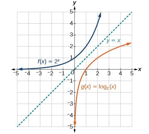
Figure 3. Notice that the graphs of [latex]f\left(x\right)={2}^{x}[/latex] and [latex]g\left(x\right)={\mathrm{log}}_{2}\left(x\right)[/latex] are reflections about the line y = x.

Observe the following from the graph:

• [latex]f\left(x\right)={2}^{x}[/latex] has a y-intercept at [latex]\left(0,1\right)[/latex] and [latex]g\left(x\right)={\mathrm{log}}_{2}\left(x\right)[/latex] has an x-intercept at [latex]\left(1,0\right)[/latex].
• The domain of [latex]f\left(x\right)={2}^{x}[/latex], [latex]\left(-\infty ,\infty \right)[/latex], is the same as the range of [latex]g\left(x\right)={\mathrm{log}}_{2}\left(x\right)[/latex].
• The range of [latex]f\left(x\right)={2}^{x}[/latex], [latex]\left(0,\infty \right)[/latex], is the same as the domain of [latex]g\left(x\right)={\mathrm{log}}_{2}\left(x\right)[/latex].

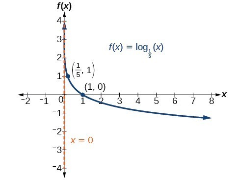
A General Note: Characteristics of the Graph of the Parent Function, f(x) = log_b(x)

For any real number x and constant b > 0, [latex]b\ne 1[/latex], we can see the following characteristics in the graph of [latex]f\left(x\right)={\mathrm{log}}_{b}\left(x\right)[/latex]:

• one-to-one function
• vertical asymptote: x = 0
• domain: [latex]\left(0,\infty \right)[/latex]
• range: [latex]\left(-\infty ,\infty \right)[/latex]
• x-intercept: [latex]\left(1,0\right)[/latex] and key point [latex]\left(b,1\right)[/latex]
• y-intercept: none
• increasing if [latex]b>1[/latex]
• decreasing if 0 < b < 1

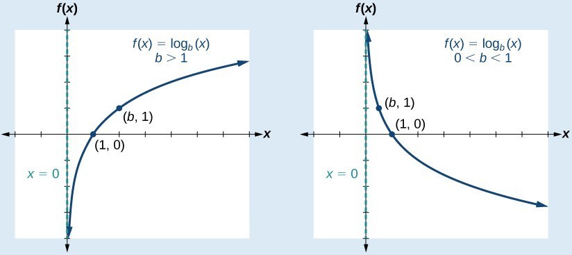
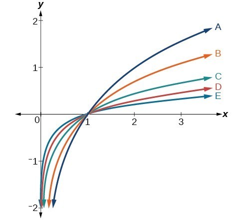
Figure 4 shows how changing the base b in [latex]f\left(x\right)={\mathrm{log}}_{b}\left(x\right)[/latex] can affect the graphs. Observe that the graphs compress vertically as the value of the base increases. (Note: recall that the function [latex]\mathrm{ln}\left(x\right)[/latex] has base [latex]e\approx \text{2}.\text{718.)}[/latex]

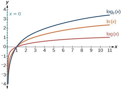
Figure 4. The graphs of three logarithmic functions with different bases, all greater than 1.

How To: Given a logarithmic function with the form [latex]f\left(x\right)={\mathrm{log}}_{b}\left(x\right)[/latex], graph the function.

1. Draw and label the vertical asymptote, x = 0.
2. Plot the x-intercept, [latex]\left(1,0\right)[/latex].
3. Plot the key point [latex]\left(b,1\right)[/latex].
4. Draw a smooth curve through the points.
5. State the domain, [latex]\left(0,\infty \right)[/latex], the range, [latex]\left(-\infty ,\infty \right)[/latex], and the vertical asymptote, x = 0.

Example 8: Graphing a Logarithmic Function with the Form [latex]f\left(x\right)={\mathrm{log}}_{b}\left(x\right)[/latex].

Graph [latex]f\left(x\right)={\mathrm{log}}_{5}\left(x\right)[/latex]. State the domain, range, and asymptote.

Show Solution

Before graphing, identify the behavior and key points for the graph.

• Since b = 5 is greater than one, we know the function is increasing. The left tail of the graph will approach the vertical asymptote x = 0, and the right tail will increase slowly without bound.
• The x-intercept is [latex]\left(1,0\right)[/latex].
• The key point [latex]\left(5,1\right)[/latex] is on the graph.
• We draw and label the asymptote, plot and label the points, and draw a smooth curve through the points.

Figure 5. The domain is [latex]\left(0,\infty \right)[/latex], the range is [latex]\left(-\infty ,\infty \right)[/latex], and the vertical asymptote is x = 0.

Try It

Graph [latex]f\left(x\right)={\mathrm{log}}_{\frac{1}{5}}\left(x\right)[/latex]. State the domain, range, and asymptote.

Show Solution

The domain is [latex]\left(0,\infty \right)[/latex], the range is [latex]\left(-\infty ,\infty \right)[/latex], and the vertical asymptote is x = 0.

Try It

 Graphing Transformations of Logarithmic Functions

As we mentioned in the beginning of the section, transformations of logarithmic graphs behave similarly to those of other parent functions. We can shift, stretch, compress, and reflect the parent function [latex]y={\mathrm{log}}_{b}\left(x\right)[/latex] without loss of shape.

Graphing a Horizontal Shift of [latex]f\left(x\right)={\mathrm{log}}_{b}\left(x\right)[/latex]

When a constant c is added to the input of the parent function [latex]f\left(x\right)=\text{log}_{b}\left(x\right)[/latex], the result is a horizontal shift c units in the opposite direction of the sign on c. To visualize horizontal shifts, we can observe the general graph of the parent function [latex]f\left(x\right)={\mathrm{log}}_{b}\left(x\right)[/latex] and for c > 0 alongside the shift left, [latex]g\left(x\right)={\mathrm{log}}_{b}\left(x+c\right)[/latex], and the shift right, [latex]h\left(x\right)={\mathrm{log}}_{b}\left(x-c\right)[/latex].

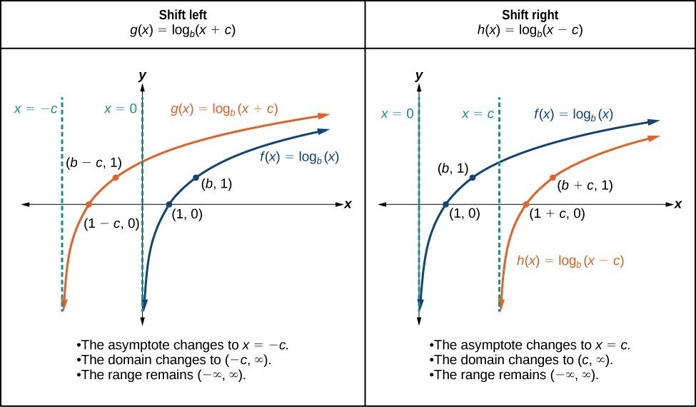
Figure 6

A General Note: Horizontal Shifts of the Parent Function [latex]y=\text{log}_{b}\left(x\right)[/latex]

For any constant c, the function [latex]f\left(x\right)={\mathrm{log}}_{b}\left(x+c\right)[/latex]

• shifts the parent function [latex]y={\mathrm{log}}_{b}\left(x\right)[/latex] left c units if c > 0.
• shifts the parent function [latex]y={\mathrm{log}}_{b}\left(x\right)[/latex] right c units if c < 0.
• has the vertical asymptote x = –c.
• has domain [latex]\left(-c,\infty \right)[/latex].
• has range [latex]\left(-\infty ,\infty \right)[/latex].

How To: Given a logarithmic function with the form [latex]f\left(x\right)={\mathrm{log}}_{b}\left(x+c\right)[/latex], graph the translation.

1. Identify the horizontal shift:
   1. If c > 0, shift the graph of [latex]f\left(x\right)={\mathrm{log}}_{b}\left(x\right)[/latex] left c units.
   2. If c < 0, shift the graph of [latex]f\left(x\right)={\mathrm{log}}_{b}\left(x\right)[/latex] right c units.
2. Draw the vertical asymptote x = –c.
3. Identify three key points from the parent function. Find new coordinates for the shifted functions by subtracting c from the x coordinate.
4. Label the three points.
5. The Domain is [latex]\left(-c,\infty \right)[/latex], the range is [latex]\left(-\infty ,\infty \right)[/latex], and the vertical asymptote is x = –c.

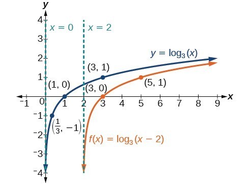
Example 9: Graphing a Horizontal Shift of the Parent Function [latex]y=\text{log}_{b}\left(x\right)[/latex]

Sketch the horizontal shift [latex]f\left(x\right)={\mathrm{log}}_{3}\left(x - 2\right)[/latex] alongside its parent function. Include the key points and asymptotes on the graph. State the domain, range, and asymptote.

Show Solution

Since the function is [latex]f\left(x\right)={\mathrm{log}}_{3}\left(x - 2\right)[/latex], we notice [latex]x+\left(-2\right)=x - 2[/latex].

Thus c = –2, so c < 0. This means we will shift the function [latex]f\left(x\right)={\mathrm{log}}_{3}\left(x\right)[/latex] right 2 units.

The vertical asymptote is [latex]x=-\left(-2\right)[/latex] or x = 2.

Consider the three key points from the parent function, [latex]\left(\frac{1}{3},-1\right)[/latex], [latex]\left(1,0\right)[/latex], and [latex]\left(3,1\right)[/latex].

The new coordinates are found by adding 2 to the x coordinates.

Label the points [latex]\left(\frac{7}{3},-1\right)[/latex], [latex]\left(3,0\right)[/latex], and [latex]\left(5,1\right)[/latex].

The domain is [latex]\left(2,\infty \right)[/latex], the range is [latex]\left(-\infty ,\infty \right)[/latex], and the vertical asymptote is x = 2.

Figure 7

 

Try It

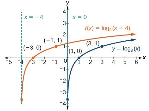
Sketch a graph of [latex]f\left(x\right)={\mathrm{log}}_{3}\left(x+4\right)[/latex] alongside its parent function. Include the key points and asymptotes on the graph. State the domain, range, and asymptote.

Show Solution

The domain is [latex]\left(-4,\infty \right)[/latex], the range [latex]\left(-\infty ,\infty \right)[/latex], and the asymptote x = –4.

Try It

Graphing a Vertical Shift of [latex]y=\text{log}_{b}\left(x\right)[/latex]

When a constant d is added to the parent function [latex]f\left(x\right)={\mathrm{log}}_{b}\left(x\right)[/latex], the result is a vertical shift d units in the direction of the sign on d. To visualize vertical shifts, we can observe the general graph of the parent function [latex]f\left(x\right)={\mathrm{log}}_{b}\left(x\right)[/latex] alongside the shift up, [latex]g\left(x\right)={\mathrm{log}}_{b}\left(x\right)+d[/latex] and the shift down, [latex]h\left(x\right)={\mathrm{log}}_{b}\left(x\right)-d[/latex].

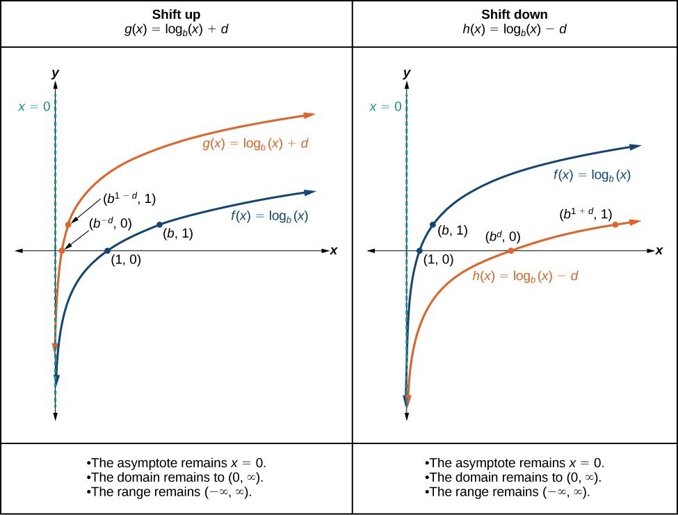
Figure 8

A General Note: Vertical Shifts of the Parent Function [latex]y=\text{log}_{b}\left(x\right)[/latex]

For any constant d, the function [latex]f\left(x\right)={\mathrm{log}}_{b}\left(x\right)+d[/latex]

• shifts the parent function [latex]y={\mathrm{log}}_{b}\left(x\right)[/latex] up d units if d > 0.
• shifts the parent function [latex]y={\mathrm{log}}_{b}\left(x\right)[/latex] down d units if d < 0.
• has the vertical asymptote x = 0.
• has domain [latex]\left(0,\infty \right)[/latex].
• has range [latex]\left(-\infty ,\infty \right)[/latex].

How To: Given a logarithmic function with the form [latex]f\left(x\right)={\mathrm{log}}_{b}\left(x\right)+d[/latex], graph the translation.

1. Identify the vertical shift:
   1. If d > 0, shift the graph of [latex]f\left(x\right)={\mathrm{log}}_{b}\left(x\right)[/latex] up d units.
   2. If d < 0, shift the graph of [latex]f\left(x\right)={\mathrm{log}}_{b}\left(x\right)[/latex] down d units.
2. Draw the vertical asymptote x = 0.
3. Identify three key points from the parent function. Find new coordinates for the shifted functions by adding d to the y coordinate.
4. Label the three points.
5. The domain is [latex]\left(0,\infty \right)[/latex], the range is [latex]\left(-\infty ,\infty \right)[/latex], and the vertical asymptote is x = 0.

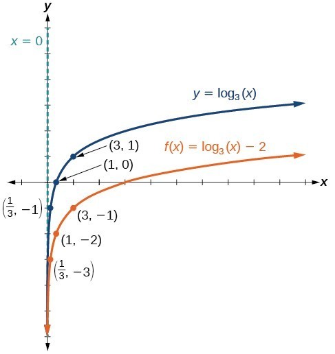
Example 10: Graphing a Vertical Shift of the Parent Function [latex]y=\text{log}_{b}\left(x\right)[/latex]

Sketch a graph of [latex]f\left(x\right)={\mathrm{log}}_{3}\left(x\right)-2[/latex] alongside its parent function. Include the key points and asymptote on the graph. State the domain, range, and asymptote.

Show Solution

Since the function is [latex]f\left(x\right)={\mathrm{log}}_{3}\left(x\right)-2[/latex], we will notice d = –2. Thus d < 0.

This means we will shift the function [latex]f\left(x\right)={\mathrm{log}}_{3}\left(x\right)[/latex] down 2 units.

The vertical asymptote is x = 0.

Consider the three key points from the parent function, [latex]\left(\frac{1}{3},-1\right)[/latex], [latex]\left(1,0\right)[/latex], and [latex]\left(3,1\right)[/latex].

The new coordinates are found by subtracting 2 from the y coordinates.

Label the points [latex]\left(\frac{1}{3},-3\right)[/latex], [latex]\left(1,-2\right)[/latex], and [latex]\left(3,-1\right)[/latex].

The domain is [latex]\left(0,\infty \right)[/latex], the range is [latex]\left(-\infty ,\infty \right)[/latex], and the vertical asymptote is x = 0.

Figure 9. The domain is [latex]\left(0,\infty \right)[/latex], the range is [latex]\left(-\infty ,\infty \right)[/latex], and the vertical asymptote is x = 0.

Try It

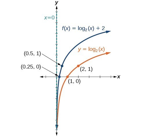
Sketch a graph of [latex]f\left(x\right)={\mathrm{log}}_{2}\left(x\right)+2[/latex] alongside its parent function. Include the key points and asymptote on the graph. State the domain, range, and asymptote.

Show Solution

The domain is [latex]\left(0,\infty \right)[/latex], the range is [latex]\left(-\infty ,\infty \right)[/latex], and the vertical asymptote is x = 0.

Try It

Graphing Stretches and Compressions of [latex]y=\text{log}_{b}\left(x\right)[/latex]

When the parent function [latex]f\left(x\right)={\mathrm{log}}_{b}\left(x\right)[/latex] is multiplied by a constant a > 0, the result is a vertical stretch or compression of the original graph. To visualize stretches and compressions, we set a > 1 and observe the general graph of the parent function [latex]f\left(x\right)={\mathrm{log}}_{b}\left(x\right)[/latex] alongside the vertical stretch, [latex]g\left(x\right)=a{\mathrm{log}}_{b}\left(x\right)[/latex] and the vertical compression, [latex]h\left(x\right)=\frac{1}{a}{\mathrm{log}}_{b}\left(x\right)[/latex].

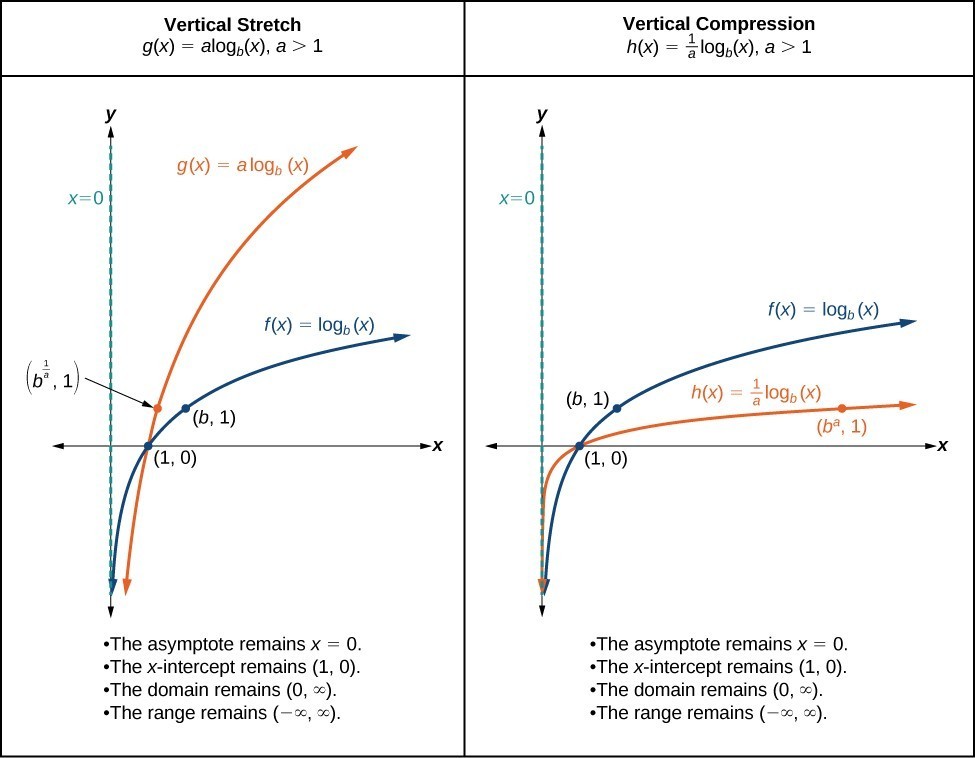
A General Note: Vertical Stretches and Compressions of the Parent Function [latex]y=\text{log}_{b}\left(x\right)[/latex]

For any constant a > 1, the function [latex]f\left(x\right)=a{\mathrm{log}}_{b}\left(x\right)[/latex]

• stretches the parent function [latex]y={\mathrm{log}}_{b}\left(x\right)[/latex] vertically by a factor of a if a > 1.
• compresses the parent function [latex]y={\mathrm{log}}_{b}\left(x\right)[/latex] vertically by a factor of a if 0 < a < 1.
• has the vertical asymptote x = 0.
• has the x-intercept [latex]\left(1,0\right)[/latex].
• has domain [latex]\left(0,\infty \right)[/latex].
• has range [latex]\left(-\infty ,\infty \right)[/latex].

How To: Given a logarithmic function with the form [latex]f\left(x\right)=a{\mathrm{log}}_{b}\left(x\right)[/latex], [latex]a>0[/latex], graph the translation.

1. Identify the vertical stretch or compressions:
   1. If [latex]|a|>1[/latex], the graph of [latex]f\left(x\right)={\mathrm{log}}_{b}\left(x\right)[/latex] is stretched by a factor of a units.
   2. If [latex]|a|<1[/latex], the graph of [latex]f\left(x\right)={\mathrm{log}}_{b}\left(x\right)[/latex] is compressed by a factor of a units.
2. Draw the vertical asymptote x = 0.
3. Identify three key points from the parent function. Find new coordinates for the shifted functions by multiplying the y coordinates by a.
4. Label the three points.
5. The domain is [latex]\left(0,\infty \right)[/latex], the range is [latex]\left(-\infty ,\infty \right)[/latex], and the vertical asymptote is x = 0.

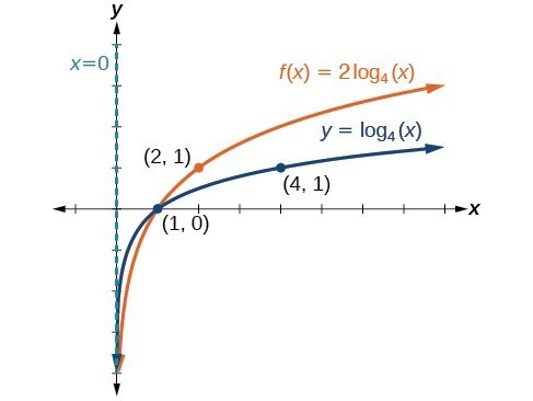
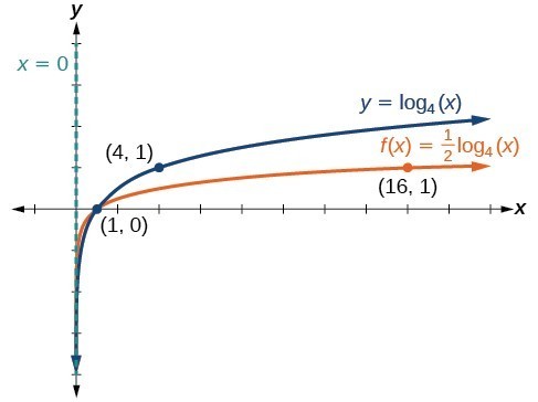
Example 11: Graphing a Stretch or Compression of the Parent Function [latex]y=\text{log}_{b}\left(x\right)[/latex]

Sketch a graph of [latex]f\left(x\right)=2{\mathrm{log}}_{4}\left(x\right)[/latex] alongside its parent function. Include the key points and asymptote on the graph. State the domain, range, and asymptote.

Show Solution

Since the function is [latex]f\left(x\right)=2{\mathrm{log}}_{4}\left(x\right)[/latex], we will notice a = 2.

This means we will stretch the function [latex]f\left(x\right)={\mathrm{log}}_{4}\left(x\right)[/latex] by a factor of 2.

The vertical asymptote is x = 0.

Consider the three key points from the parent function, [latex]\left(\frac{1}{4},-1\right)[/latex], [latex]\left(1,0\right)[/latex], and [latex]\left(4,1\right)[/latex].

The new coordinates are found by multiplying the y coordinates by 2.

Label the points [latex]\left(\frac{1}{4},-2\right)[/latex], [latex]\left(1,0\right)[/latex], and [latex]\left(4,\text{2}\right)[/latex].

The domain is [latex]\left(0,\infty \right)[/latex], the range is [latex]\left(-\infty ,\infty \right)[/latex], and the vertical asymptote is x = 0.

Figure 11. The domain is [latex]\left(0,\infty \right)[/latex], the range is [latex]\left(-\infty ,\infty \right)[/latex], and the vertical asymptote is x = 0.

Try It

Sketch a graph of [latex]f\left(x\right)=\frac{1}{2}{\mathrm{log}}_{4}\left(x\right)[/latex] alongside its parent function. Include the key points and asymptote on the graph. State the domain, range, and asymptote.

Show Solution

The domain is [latex]\left(0,\infty \right)[/latex], the range is [latex]\left(-\infty ,\infty \right)[/latex], and the vertical asymptote is x = 0.

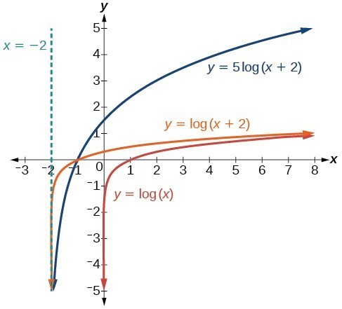
Example 12: Combining a Shift and a Stretch

Sketch a graph of [latex]f\left(x\right)=5\mathrm{log}\left(x+2\right)[/latex]. State the domain, range, and asymptote.

Show Solution

Remember: what happens inside parentheses happens first. First, we move the graph left 2 units, then stretch the function vertically by a factor of 5. The vertical asymptote will be shifted to x = –2. The x-intercept will be [latex]\left(-1,0\right)[/latex]. The domain will be [latex]\left(-2,\infty \right)[/latex]. Two points will help give the shape of the graph: [latex]\left(-1,0\right)[/latex] and [latex]\left(8,5\right)[/latex]. We chose x = 8 as the x-coordinate of one point to graph because when x = 8, x + 2 = 10, the base of the common logarithm.

Figure 12. The domain is [latex]\left(-2,\infty \right)[/latex], the range is [latex]\left(-\infty ,\infty \right)[/latex], and the vertical asymptote is x = –2.

Try It

Sketch a graph of the function [latex]f\left(x\right)=3\mathrm{log}\left(x - 2\right)+1[/latex]. State the domain, range, and asymptote.

Show Solution

The domain is [latex]\left(2,\infty \right)[/latex], the range is [latex]\left(-\infty ,\infty \right)[/latex], and the vertical asymptote is x = 2.

Try It

Graphing Reflections of [latex]f\left(x\right)={\mathrm{log}}_{b}\left(x\right)[/latex]

When the parent function [latex]f\left(x\right)={\mathrm{log}}_{b}\left(x\right)[/latex] is multiplied by –1, the result is a reflection about the x-axis. When the input is multiplied by –1, the result is a reflection about the y-axis. To visualize reflections, we restrict b > 1, and observe the general graph of the parent function [latex]f\left(x\right)={\mathrm{log}}_{b}\left(x\right)[/latex] alongside the reflection about the x-axis, [latex]g\left(x\right)={\mathrm{-log}}_{b}\left(x\right)[/latex] and the reflection about the y-axis, [latex]h\left(x\right)={\mathrm{log}}_{b}\left(-x\right)[/latex].

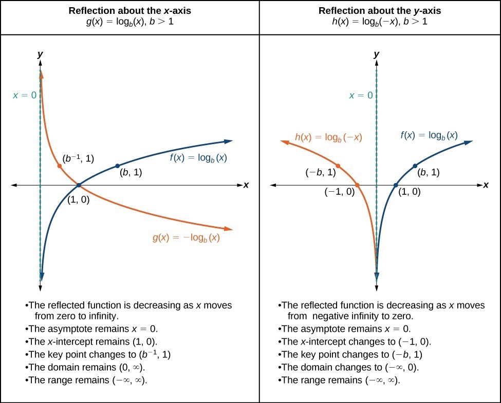
A General Note: Reflections of the Parent Function [latex]y=\text{log}_{b}\left(x\right)[/latex]

The function [latex]f\left(x\right)={\mathrm{-log}}_{b}\left(x\right)[/latex]

• reflects the parent function [latex]y={\mathrm{log}}_{b}\left(x\right)[/latex] about the x-axis.
• has domain, [latex]\left(0,\infty \right)[/latex], range, [latex]\left(-\infty ,\infty \right)[/latex], and vertical asymptote, x = 0, which are unchanged from the parent function.

The function [latex]f\left(x\right)={\mathrm{log}}_{b}\left(-x\right)[/latex]

• reflects the parent function [latex]y={\mathrm{log}}_{b}\left(x\right)[/latex] about the y-axis.
• has domain [latex]\left(-\infty ,0\right)[/latex].
• has range, [latex]\left(-\infty ,\infty \right)[/latex], and vertical asymptote, x = 0, which are unchanged from the parent function.

How To: Given a logarithmic function with the parent function [latex]f\left(x\right)={\mathrm{log}}_{b}\left(x\right)[/latex], graph a translation.

[latex]\text{If }f\left(x\right)=-{\mathrm{log}}_{b}\left(x\right)[/latex]	[latex]\text{If }f\left(x\right)={\mathrm{log}}_{b}\left(-x\right)[/latex]
1. Draw the vertical asymptote, x = 0.	1. Draw the vertical asymptote, x = 0.
2. Plot the x-intercept, [latex]\left(1,0\right)[/latex].	2. Plot the x-intercept, [latex]\left(1,0\right)[/latex].
3. Reflect the graph of the parent function [latex]f\left(x\right)={\mathrm{log}}_{b}\left(x\right)[/latex] about the x-axis.	3. Reflect the graph of the parent function [latex]f\left(x\right)={\mathrm{log}}_{b}\left(x\right)[/latex] about the y-axis.
4. Draw a smooth curve through the points.	4. Draw a smooth curve through the points.
5. State the domain, [latex]\left(0,\infty \right)[/latex], the range, [latex]\left(-\infty ,\infty \right)[/latex], and the vertical asymptote x = 0.	5. State the domain, [latex]\left(-\infty ,0\right)[/latex], the range, [latex]\left(-\infty ,\infty \right)[/latex], and the vertical asymptote x = 0.

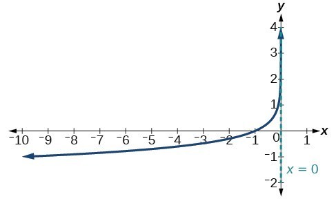
Example 13: Graphing a Reflection of a Logarithmic Function

Sketch a graph of [latex]f\left(x\right)=\mathrm{log}\left(-x\right)[/latex] alongside its parent function. Include the key points and asymptote on the graph. State the domain, range, and asymptote.

Show Solution

Before graphing [latex]f\left(x\right)=\mathrm{log}\left(-x\right)[/latex], identify the behavior and key points for the graph.

• Since b = 10 is greater than one, we know that the parent function is increasing. Since the input value is multiplied by –1, f is a reflection of the parent graph about the y-axis. Thus, [latex]f\left(x\right)=\mathrm{log}\left(-x\right)[/latex] will be decreasing as x moves from negative infinity to zero, and the right tail of the graph will approach the vertical asymptote x = 0.
• The x-intercept is [latex]\left(-1,0\right)[/latex].
• We draw and label the asymptote, plot and label the points, and draw a smooth curve through the points.

Figure 14. The domain is [latex]\left(-\infty ,0\right)[/latex], the range is [latex]\left(-\infty ,\infty \right)[/latex], and the vertical asymptote is x = 0.

Try It

Graph [latex]f\left(x\right)=-\mathrm{log}\left(-x\right)[/latex]. State the domain, range, and asymptote.

Show Solution

The domain is [latex]\left(-\infty ,0\right)[/latex], the range is [latex]\left(-\infty ,\infty \right)[/latex], and the vertical asymptote is x = 0.

 

Summarizing Translations of the Logarithmic Function

Now that we have worked with each type of translation for the logarithmic function, we can summarize each in the table below to arrive at the general equation for translating exponential functions.

Translations of the Parent Function [latex]y={\mathrm{log}}_{b}\left(x\right)[/latex]
Translation	Form
Shift Horizontally c units to the left Vertically d units up	[latex]y={\mathrm{log}}_{b}\left(x+c\right)+d[/latex]
Stretch and Compress Stretch if [latex]|a|>1[/latex] Compression if [latex]|a|<1[/latex]	[latex]y=a{\mathrm{log}}_{b}\left(x\right)[/latex]
Reflect about the x-axis	[latex]y=-{\mathrm{log}}_{b}\left(x\right)[/latex]
Reflect about the y-axis	[latex]y={\mathrm{log}}_{b}\left(-x\right)[/latex]
General equation for all translations	[latex]y=a{\mathrm{log}}_{b}\left(x+c\right)+d[/latex]

A General Note: Translations of Logarithmic Functions

All translations of the parent logarithmic function, [latex]y={\mathrm{log}}_{b}\left(x\right)[/latex], have the form

[latex] f\left(x\right)=a{\mathrm{log}}_{b}\left(x+c\right)+d[/latex]

where the parent function, [latex]y={\mathrm{log}}_{b}\left(x\right),b>1[/latex], is

• shifted vertically up d units.
• shifted horizontally to the left c units.
• stretched vertically by a factor of |a| if |a| > 0.
• compressed vertically by a factor of |a| if 0 < |a| < 1.
• reflected about the x-axis when a < 0.

For [latex]f\left(x\right)=\mathrm{log}\left(-x\right)[/latex], the graph of the parent function is reflected about the y-axis.

Example 14: Finding the Vertical Asymptote of a Logarithm Graph

What is the vertical asymptote of [latex]f\left(x\right)=-2{\mathrm{log}}_{3}\left(x+4\right)+5[/latex]?

Show Solution

The vertical asymptote is at x = –4.

Analysis of the Solution

The coefficient, the base, and the upward translation do not affect the asymptote. The shift of the curve 4 units to the left shifts the vertical asymptote to x = –4.

Try It

What is the vertical asymptote of [latex]f\left(x\right)=3+\mathrm{ln}\left(x - 1\right)[/latex]?

Show Solution

x = 1

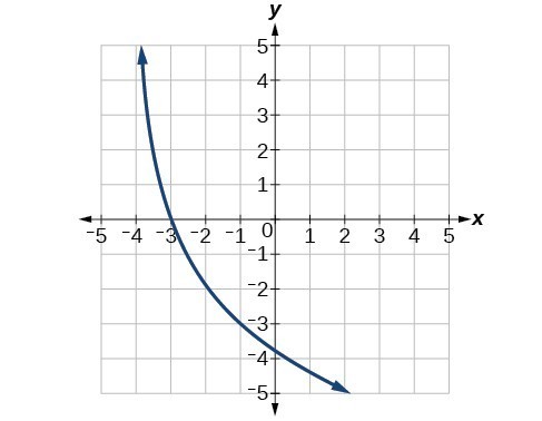
Example 15: Finding the Equation from a Graph

Find a possible equation for the common logarithmic function graphed in Figure 15.

Figure 15

Show Solution

This graph has a vertical asymptote at x = –2 and has been vertically reflected. We do not know yet the vertical shift or the vertical stretch. We know so far that the equation will have form:

[latex]f\left(x\right)=-a\mathrm{log}\left(x+2\right)+k[/latex]

It appears the graph passes through the points [latex]\left(-1,1\right)[/latex] and [latex]\left(2,-1\right)[/latex]. Substituting [latex]\left(-1,1\right)[/latex],

[latex]\begin{align}&1=-a\mathrm{log}\left(-1+2\right)+k && \text{Substitute }\left(-1,1\right). \\ &1=-a\mathrm{log}\left(1\right)+k && \text{Arithmetic}. \\ &1=k && \text{log(1)}=0. \end{align}[/latex]

Next, substituting in [latex]\left(2,-1\right)[/latex],

[latex]\begin{align}&-1=-a\mathrm{log}\left(2+2\right)+1 && \text{Plug in }\left(2,-1\right). \\ &-2=-a\mathrm{log}\left(4\right) && \text{Arithmetic}. \\ &a=\frac{2}{\mathrm{log}\left(4\right)}&& \text{Solve for }a. \end{align}[/latex]

This gives us the equation [latex]f\left(x\right)=-\frac{2}{\mathrm{log}\left(4\right)}\mathrm{log}\left(x+2\right)+1[/latex].

Analysis of the Solution

We can verify this answer by comparing the function values in the table below with the points on the graph in Example 11.

x	−1	0	1	2	3
f(x)	1	0	−0.58496	−1	−1.3219
x	4	5	6	7	8
f(x)	−1.5850	−1.8074	−2	−2.1699	−2.3219

Try It

Give the equation of the natural logarithm graphed in Figure 16.

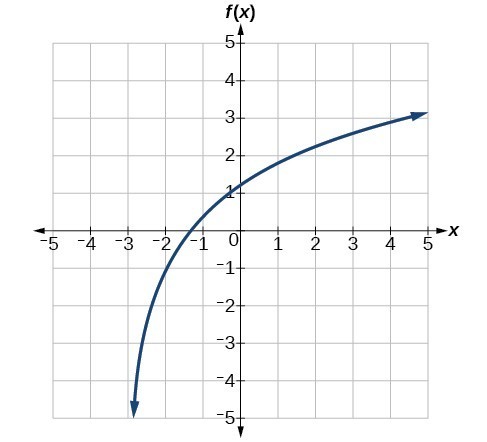
Figure 16

Show Solution

[latex]f\left(x\right)=2\mathrm{ln}\left(x+3\right)-1[/latex]

Q & A

Is it possible to tell the domain and range and describe the end behavior of a function just by looking at the graph?

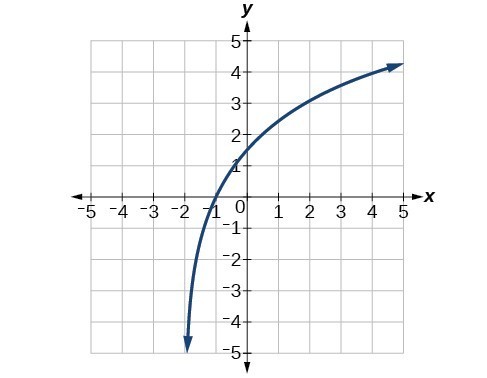
Yes, if we know the function is a general logarithmic function. For example, look at the graph in Try It 11. The graph approaches x = –3 (or thereabouts) more and more closely, so x = –3 is, or is very close to, the vertical asymptote. It approaches from the right, so the domain is all points to the right, [latex]\left\{x|x>-3\right\}[/latex]. The range, as with all general logarithmic functions, is all real numbers. And we can see the end behavior because the graph goes down as it goes left and up as it goes right. The end behavior is that as [latex]x\to -{3}^{+},f\left(x\right)\to -\infty [/latex] and as [latex]x\to \infty ,f\left(x\right)\to \infty [/latex].

Key Equations

General Form for the Translation of the Parent Logarithmic Function [latex]\text{ }f\left(x\right)={\mathrm{log}}_{b}\left(x\right)[/latex]

[latex] f\left(x\right)=a{\mathrm{log}}_{b}\left(x+c\right)+d[/latex]

Key Concepts

• The inverse of an exponential function is a logarithmic function, and the inverse of a logarithmic function is an exponential function.
• Logarithmic equations can be written in an equivalent exponential form, using the definition of a logarithm.
• Exponential equations can be written in their equivalent logarithmic form using the definition of a logarithm.
• Logarithmic functions with base b can be evaluated mentally using previous knowledge of powers of b.
• Common logarithms can be evaluated mentally using previous knowledge of powers of 10.
• When common logarithms cannot be evaluated mentally, a calculator can be used.
• Real-world exponential problems with base 10 can be rewritten as a common logarithm and then evaluated using a calculator.
• Natural logarithms can be evaluated using a calculator.
• To find the domain of a logarithmic function, set up an inequality showing the argument greater than zero, and solve for x.
• The graph of the parent function [latex]f\left(x\right)={\mathrm{log}}_{b}\left(x\right)[/latex] has an x-intercept at [latex]\left(1,0\right)[/latex], domain [latex]\left(0,\infty \right)[/latex], range [latex]\left(-\infty ,\infty \right)[/latex], vertical asymptote x = 0, and
  • if b > 1, the function is increasing.
  • if 0 < b < 1, the function is decreasing.
• The equation [latex]f\left(x\right)={\mathrm{log}}_{b}\left(x+c\right)[/latex] shifts the parent function [latex]y={\mathrm{log}}_{b}\left(x\right)[/latex] horizontally
  • left c units if c > 0.
  • right c units if c < 0.
• The equation [latex]f\left(x\right)={\mathrm{log}}_{b}\left(x\right)+d[/latex] shifts the parent function [latex]y={\mathrm{log}}_{b}\left(x\right)[/latex] vertically
  • up d units if d > 0.
  • down d units if d < 0.
• For any constant a > 0, the equation [latex]f\left(x\right)=a{\mathrm{log}}_{b}\left(x\right)[/latex]
  • stretches the parent function [latex]y={\mathrm{log}}_{b}\left(x\right)[/latex] vertically by a factor of a if |a| > 1.
  • compresses the parent function [latex]y={\mathrm{log}}_{b}\left(x\right)[/latex] vertically by a factor of a if |a| < 1.
• When the parent function [latex]y={\mathrm{log}}_{b}\left(x\right)[/latex] is multiplied by –1, the result is a reflection about the x-axis. When the input is multiplied by –1, the result is a reflection about the y-axis.
  • The equation [latex]f\left(x\right)=-{\mathrm{log}}_{b}\left(x\right)[/latex] represents a reflection of the parent function about the x-axis.
  • The equation [latex]f\left(x\right)={\mathrm{log}}_{b}\left(-x\right)[/latex] represents a reflection of the parent function about the y-axis.
  • A graphing calculator may be used to approximate solutions to some logarithmic equations.
• All translations of the logarithmic function can be summarized by the general equation [latex] f\left(x\right)=a{\mathrm{log}}_{b}\left(x+c\right)+d[/latex].
• Given an equation with the general form [latex] f\left(x\right)=a{\mathrm{log}}_{b}\left(x+c\right)+d[/latex], we can identify the vertical asymptote x = –c for the transformation.
• Using the general equation [latex]f\left(x\right)=a{\mathrm{log}}_{b}\left(x+c\right)+d[/latex], we can write the equation of a logarithmic function given its graph.

Glossary

common logarithm

the exponent to which 10 must be raised to get x; [latex]{\mathrm{log}}_{10}\left(x\right)[/latex] is written simply as [latex]\mathrm{log}\left(x\right)[/latex].

logarithm

the exponent to which b must be raised to get x; written [latex]y={\mathrm{log}}_{b}\left(x\right)[/latex]

natural logarithm

the exponent to which the number e must be raised to get x; [latex]{\mathrm{log}}_{e}\left(x\right)[/latex] is written as [latex]\mathrm{ln}\left(x\right)[/latex].

 

Section 3.2 Homework Exercises

1. What is a base b logarithm? Discuss the meaning by interpreting each part of the equivalent equations [latex]{b}^{y}=x[/latex] and [latex]{\mathrm{log}}_{b}x=y[/latex] for [latex]b>0,b\ne 1[/latex].

2. How is the logarithmic function [latex]f\left(x\right)={\mathrm{log}}_{b}x[/latex] related to the exponential function [latex]g\left(x\right)={b}^{x}[/latex]? What is the result of composing these two functions?

3. How can the logarithmic equation [latex]{\mathrm{log}}_{b}x=y[/latex] be solved for x using the properties of exponents?

4. Discuss the meaning of the common logarithm. What is its relationship to a logarithm with base b, and how does the notation differ?

5. Discuss the meaning of the natural logarithm. What is its relationship to a logarithm with base b, and how does the notation differ?

6. What type(s) of translation(s), if any, affect the range of a logarithmic function?

7. The inverse of every logarithmic function is an exponential function and vice-versa. What does this tell us about the relationship between the coordinates of the points on the graphs of each?

8. Consider the general logarithmic function [latex]f\left(x\right)={\mathrm{log}}_{b}\left(x\right)[/latex]. Why can’t x be zero?

9. Does the graph of a general logarithmic function have a horizontal asymptote? Explain.

For the following exercises, rewrite each equation in exponential form.

10. [latex]{\text{log}}_{4}\left(q\right)=m[/latex]

11. [latex]{\text{log}}_{a}\left(b\right)=c[/latex]

12. [latex]{\mathrm{log}}_{16}\left(y\right)=x[/latex]

13. [latex]{\mathrm{log}}_{x}\left(64\right)=y[/latex]

14. [latex]{\mathrm{log}}_{y}\left(x\right)=-11[/latex]

15. [latex]{\mathrm{log}}_{15}\left(a\right)=b[/latex]

16. [latex]{\mathrm{log}}_{y}\left(137\right)=x[/latex]

17. [latex]{\mathrm{log}}_{13}\left(142\right)=a[/latex]

18. [latex]\text{log}\left(v\right)=t[/latex]

19. [latex]\text{ln}\left(w\right)=n[/latex]

For the following exercises, rewrite each equation in logarithmic form.

20. [latex]{4}^{x}=y[/latex]

21. [latex]{c}^{d}=k[/latex]

22. [latex]{m}^{-7}=n[/latex]

23. [latex]{19}^{x}=y[/latex]

24. [latex]{x}^{-\frac{10}{13}}=y[/latex]

25. [latex]{n}^{4}=103[/latex]

26. [latex]{\left(\frac{7}{5}\right)}^{m}=n[/latex]

27. [latex]{y}^{x}=\frac{39}{100}[/latex]

28. [latex]{10}^{a}=b[/latex]

29. [latex]{e}^{k}=h[/latex]

For the following exercises, solve for x by converting the logarithmic equation to exponential form.

30. [latex]{\text{log}}_{3}\left(x\right)=2[/latex]

31. [latex]{\text{log}}_{2}\left(x\right)=-3[/latex]

32. [latex]{\text{log}}_{5}\left(x\right)=2[/latex]

33. [latex]{\mathrm{log}}_{3}\left(x\right)=3[/latex]

34. [latex]{\text{log}}_{2}\left(x\right)=6[/latex]

35. [latex]{\text{log}}_{9}\left(x\right)=\frac{1}{2}[/latex]

36. [latex]{\text{log}}_{18}\left(x\right)=2[/latex]

37. [latex]{\mathrm{log}}_{6}\left(x\right)=-3[/latex]

38. [latex]\text{log}\left(x\right)=3[/latex]

39. [latex]\text{ln}\left(x\right)=2[/latex]

For the following exercises, use the definition of common and natural logarithms to simplify.

40. [latex]\text{log}\left({100}^{8}\right)[/latex]

41. [latex]{10}^{\text{log}\left(32\right)}[/latex]

42. [latex]2\text{log}\left(.0001\right)[/latex]

43. [latex]{e}^{\mathrm{ln}\left(1.06\right)}[/latex]

44. [latex]\mathrm{ln}\left({e}^{-5.03}\right)[/latex]

45. [latex]{e}^{\mathrm{ln}\left(10.125\right)}+4[/latex]

For the following exercises, evaluate the base b logarithmic expression without using a calculator.

46. [latex]{\text{log}}_{3}\left(\frac{1}{27}\right)[/latex]

47. [latex]{\text{log}}_{6}\left(\sqrt{6}\right)[/latex]

48. [latex]{\text{log}}_{2}\left(\frac{1}{8}\right)+4[/latex]

49. [latex]6{\text{log}}_{8}\left(4\right)[/latex]

For the following exercises, evaluate the common logarithmic expression without using a calculator.

50. [latex]\text{log}\left(10,000\right)[/latex]

51. [latex]\text{log}\left(0.001\right)[/latex]

52. [latex]\text{log}\left(1\right)+7[/latex]

53. [latex]2\text{log}\left({100}^{-3}\right)[/latex]

For the following exercises, evaluate the natural logarithmic expression without using a calculator.

54. [latex]\text{ln}\left({e}^{\frac{1}{3}}\right)[/latex]

55. [latex]\text{ln}\left(1\right)[/latex]

56. [latex]\text{ln}\left({e}^{-0.225}\right)-3[/latex]

57. [latex]25\text{ln}\left({e}^{\frac{2}{5}}\right)[/latex]

For the following exercises, evaluate each expression using a calculator. Round to the nearest thousandth.

58. [latex]\text{log}\left(0.04\right)[/latex]

59. [latex]\text{ln}\left(15\right)[/latex]

60. [latex]\text{ln}\left(\frac{4}{5}\right)[/latex]

61. [latex]\text{log}\left(\sqrt{2}\right)[/latex]

For the following exercises, state the domain and range of the function.

62. [latex]f\left(x\right)={\mathrm{log}}_{3}\left(x+4\right)[/latex]

63. [latex]h\left(x\right)=\mathrm{ln}\left(\frac{1}{2}-x\right)[/latex]

64. [latex]g\left(x\right)={\mathrm{log}}_{5}\left(2x+9\right)-2[/latex]

65. [latex]h\left(x\right)=\mathrm{ln}\left(4x+17\right)-5[/latex]

66. [latex]f\left(x\right)={\mathrm{log}}_{2}\left(12 - 3x\right)-3[/latex]

For the following exercises, state the domain and the vertical asymptote of the function.

67. [latex]f\left(x\right)={\mathrm{log}}_{b}\left(x - 5\right)[/latex]

68. [latex]g\left(x\right)=\mathrm{ln}\left(3-x\right)[/latex]

69. [latex]f\left(x\right)=\mathrm{log}\left(3x+1\right)[/latex]

70. [latex]f\left(x\right)=3\mathrm{log}\left(-x\right)+2[/latex]

71. [latex]g\left(x\right)=-\mathrm{ln}\left(3x+9\right)-7[/latex]

For the following exercises, state the domain, vertical asymptote, and end behavior of the function.

72. [latex]f\left(x\right)=\mathrm{ln}\left(2-x\right)[/latex]

73. [latex]f\left(x\right)=\mathrm{log}\left(x-\frac{3}{7}\right)[/latex]

74. [latex]h\left(x\right)=-\mathrm{log}\left(3x - 4\right)+3[/latex]

75. [latex]g\left(x\right)=\mathrm{ln}\left(2x+6\right)-5[/latex]

76. [latex]f\left(x\right)={\mathrm{log}}_{3}\left(15 - 5x\right)+6[/latex]

For the following exercises, state the domain, range, and x- and y-intercepts, if they exist. If they do not exist, write DNE.

77. [latex]h\left(x\right)={\mathrm{log}}_{4}\left(x - 1\right)+1[/latex]

78. [latex]f\left(x\right)=\mathrm{log}\left(5x+10\right)+3[/latex]

79. [latex]g\left(x\right)=\mathrm{ln}\left(-x\right)-2[/latex]

80. [latex]f\left(x\right)={\mathrm{log}}_{2}\left(x+2\right)-5[/latex]

81. [latex]h\left(x\right)=3\mathrm{ln}\left(x\right)-9[/latex]

For the following exercises, match each function in the graph below with the letter corresponding to its graph.

82. [latex]d\left(x\right)=\mathrm{log}\left(x\right)[/latex]

83. [latex]f\left(x\right)=\mathrm{ln}\left(x\right)[/latex]

84. [latex]g\left(x\right)={\mathrm{log}}_{2}\left(x\right)[/latex]

85. [latex]h\left(x\right)={\mathrm{log}}_{5}\left(x\right)[/latex]

86. [latex]j\left(x\right)={\mathrm{log}}_{25}\left(x\right)[/latex]

For the following exercises, match each function in the figure below with the letter corresponding to its graph.

87. [latex]f\left(x\right)={\mathrm{log}}_{\frac{1}{3}}\left(x\right)[/latex]

88. [latex]g\left(x\right)={\mathrm{log}}_{2}\left(x\right)[/latex]

89. [latex]h\left(x\right)={\mathrm{log}}_{\frac{3}{4}}\left(x\right)[/latex]

For the following exercises, sketch the graphs of each pair of functions on the same axis.

90. [latex]f\left(x\right)=\mathrm{log}\left(x\right)[/latex] and [latex]g\left(x\right)={10}^{x}[/latex]

91. [latex]f\left(x\right)=\mathrm{log}\left(x\right)[/latex] and [latex]g\left(x\right)={\mathrm{log}}_{\frac{1}{2}}\left(x\right)[/latex]

92. [latex]f\left(x\right)={\mathrm{log}}_{4}\left(x\right)[/latex] and [latex]g\left(x\right)=\mathrm{ln}\left(x\right)[/latex]

93. [latex]f\left(x\right)={e}^{x}[/latex] and [latex]g\left(x\right)=\mathrm{ln}\left(x\right)[/latex]

For the following exercises, match each function in the graph below with the letter corresponding to its graph.

94. [latex]f\left(x\right)={\mathrm{log}}_{4}\left(-x+2\right)[/latex]

95. [latex]g\left(x\right)=-{\mathrm{log}}_{4}\left(x+2\right)[/latex]

96. [latex]h\left(x\right)={\mathrm{log}}_{4}\left(x+2\right)[/latex]

For the following exercises, sketch the graph of the indicated function.

97. [latex]f\left(x\right)={\mathrm{log}}_{2}\left(x+2\right)[/latex]

98. [latex]f\left(x\right)=2\mathrm{log}\left(x\right)[/latex]

99. [latex]f\left(x\right)=\mathrm{ln}\left(-x\right)[/latex]

100. [latex]g\left(x\right)=\mathrm{log}\left(4x+16\right)+4[/latex]

101. [latex]g\left(x\right)=\mathrm{log}\left(6 - 3x\right)+1[/latex]

102. [latex]h\left(x\right)=-\frac{1}{2}\mathrm{ln}\left(x+1\right)-3[/latex]

For the following exercises, write a logarithmic equation corresponding to the graph shown.

103. Use [latex]y={\mathrm{log}}_{2}\left(x\right)[/latex] as the parent function.

104. Use [latex]f\left(x\right)={\mathrm{log}}_{3}\left(x\right)[/latex] as the parent function.

105. Use [latex]f\left(x\right)={\mathrm{log}}_{4}\left(x\right)[/latex] as the parent function.

106. Use [latex]f\left(x\right)={\mathrm{log}}_{5}\left(x\right)[/latex] as the parent function.

107. Explore and discuss the graphs of [latex]f\left(x\right)={\mathrm{log}}_{\frac{1}{2}}\left(x\right)[/latex] and [latex]g\left(x\right)=-{\mathrm{log}}_{2}\left(x\right)[/latex]. Make a conjecture based on the result.

108. Prove the conjecture made in the previous exercise.

109. What is the domain of the function [latex]f\left(x\right)=\mathrm{ln}\left(\frac{x+2}{x - 4}\right)[/latex]? Discuss the result.

110. Use properties of exponents to find the x-intercepts of the function [latex]f\left(x\right)=\mathrm{log}\left({x}^{2}+4x+4\right)[/latex] algebraically. Show the steps for solving, and then verify the result by graphing the function.

111. Is x = 0 in the domain of the function [latex]f\left(x\right)=\mathrm{log}\left(x\right)[/latex]? If so, what is the value of the function when x = 0? Verify the result.

112. Is [latex]f\left(x\right)=0[/latex] in the range of the function [latex]f\left(x\right)=\mathrm{log}\left(x\right)[/latex]? If so, for what value of x? Verify the result.

113. Is there a number x such that [latex]\mathrm{ln}x=2[/latex]? If so, what is that number? Verify the result.

114. Is the following true: [latex]\frac{{\mathrm{log}}_{3}\left(27\right)}{{\mathrm{log}}_{4}\left(\frac{1}{64}\right)}=-1[/latex]? Verify the result.

115. Is the following true: [latex]\frac{\mathrm{ln}\left({e}^{1.725}\right)}{\mathrm{ln}\left(1\right)}=1.725[/latex]? Verify the result.

116. The exposure index EI for a 35 millimeter camera is a measurement of the amount of light that hits the film. It is determined by the equation [latex]EI={\mathrm{log}}_{2}\left(\frac{{f}^{2}}{t}\right)[/latex], where f is the “f-stop” setting on the camera, and t is the exposure time in seconds. Suppose the f-stop setting is 8 and the desired exposure time is 2 seconds. What will the resulting exposure index be?

117. Refer to the previous exercise. Suppose the light meter on a camera indicates an EI of –2, and the desired exposure time is 16 seconds. What should the f-stop setting be?

118. The intensity levels I of two earthquakes measured on a seismograph can be compared by the formula [latex]\mathrm{log}\frac{{I}_{1}}{{I}_{2}}={M}_{1}-{M}_{2}[/latex] where M is the magnitude given by the Richter Scale. In August 2009, an earthquake of magnitude 6.1 hit Honshu, Japan. In March 2011, that same region experienced yet another, more devastating earthquake, this time with a magnitude of 9.0.^[5] How many times greater was the intensity of the 2011 earthquake? Round to the nearest whole number.

---