Learning Outcomes
- Use arrow notation.
- Graph rational functions.
Suppose we know that the cost of making a product is dependent on the number of items, x, produced. This is given by the equation [latex]C\left(x\right)=15,000x - 0.1{x}^{2}+1000[/latex]. If we want to know the average cost for producing x items, we would divide the cost function by the number of items, x.
The average cost function, which yields the average cost per item for x items produced, is
Many other application problems require finding an average value in a similar way, giving us variables in the denominator. Written without a variable in the denominator, this function will contain a negative integer power.
In the last few sections, we have worked with polynomial functions, which are functions with non-negative integers for exponents. In this section, we explore rational functions, which have variables in the denominator.
Use arrow notation
We have seen the graphs of the basic reciprocal function and the squared reciprocal function from our study of basic functions. Examine these graphs and notice some of their features.
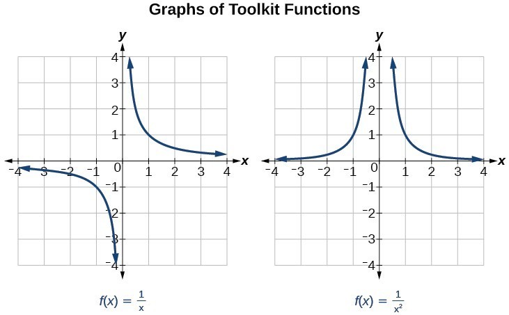
Figure 1
Several things are apparent if we examine the graph of [latex]f\left(x\right)=\frac{1}{x}[/latex].
- On the left branch of the graph, the curve approaches the x-axis [latex]\left(y=0\right) \text{ as } x\to -\infty[/latex].
- As the graph approaches [latex]x=0[/latex] from the left, the curve drops, but as we approach zero from the right, the curve rises.
- Finally, on the right branch of the graph, the curves approaches the x-axis [latex]\left(y=0\right) \text{ as } x\to \infty[/latex].
To summarize, we use arrow notation to show that x or [latex]f\left(x\right)[/latex] is approaching a particular value.
| Arrow Notation |
|
| Symbol | Meaning |
| [latex]x\to {a}^{-}[/latex] | x approaches a from the left (x < a but close to a) |
| [latex]x\to {a}^{+}[/latex] | x approaches a from the right (x > a but close to a) |
| [latex]x\to \infty\\[/latex] | x approaches infinity (x increases without bound) |
| [latex]x\to -\infty[/latex] | x approaches negative infinity (x decreases without bound) |
| [latex]f\left(x\right)\to \infty[/latex] | the output approaches infinity (the output increases without bound) |
| [latex]f\left(x\right)\to -\infty[/latex] | the output approaches negative infinity (the output decreases without bound) |
| [latex]f\left(x\right)\to a[/latex] | the output approaches a |
Local Behavior of [latex]f\left(x\right)=\frac{1}{x}[/latex]
Let’s begin by looking at the reciprocal function, [latex]f\left(x\right)=\frac{1}{x}[/latex]. We cannot divide by zero, which means the function is undefined at [latex]x=0[/latex]; so zero is not in the domain. As the input values approach zero from the left side (becoming very small, negative values), the function values decrease without bound (in other words, they approach negative infinity). We can see this behavior in the table below.
| x | –0.1 | –0.01 | –0.001 | –0.0001 |
| [latex]f\left(x\right)=\frac{1}{x}[/latex] | –10 | –100 | –1000 | –10,000 |
We write in arrow notation
As the input values approach zero from the right side (becoming very small, positive values), the function values increase without bound (approaching infinity). We can see this behavior in the table below.
| x | 0.1 | 0.01 | 0.001 | 0.0001 |
| [latex]f\left(x\right)=\frac{1}{x}[/latex] | 10 | 100 | 1000 | 10,000 |
We write in arrow notation
[latex]\text{As }x\to {0}^{+}, f\left(x\right)\to \infty[/latex].
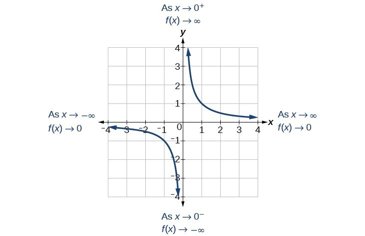
Figure 2
This behavior creates a vertical asymptote, which is a vertical line that the graph approaches but never crosses. In this case, the graph is approaching the vertical line x = 0 as the input becomes close to zero.
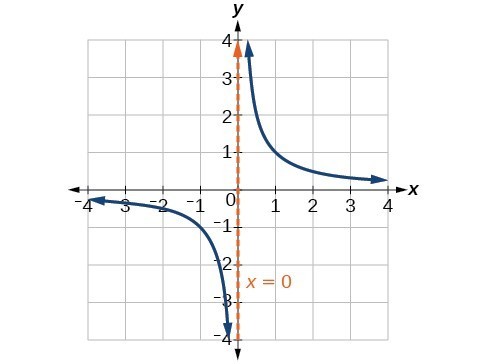
Figure 3
A General Note: Vertical Asymptote
A vertical asymptote of a graph is a vertical line [latex]x=a[/latex] where the graph tends toward positive or negative infinity as the inputs approach a. We write
Example 1: Using Arrow Notation
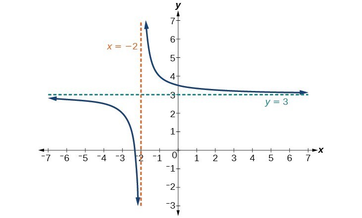
Use arrow notation to describe the end behavior and local behavior of the function graphed in Figure 4.
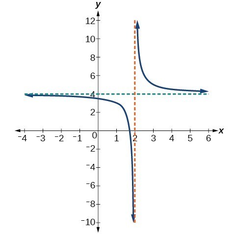
Figure 4
Try It
Use arrow notation to describe the end behavior and local behavior for the reciprocal squared function, [latex]f(x)=\frac{1}{x^2}[/latex].
Example 2: Using Transformations to Graph a Rational Function
Sketch a graph of the reciprocal function shifted two units to the left and up three units. Identify the horizontal and vertical asymptotes of the graph, if any.
Try It
Sketch the graph, and find the horizontal and vertical asymptotes of the reciprocal squared function that has been shifted right 3 units and down 4 units.

Graph rational functions
We have previously stated that the numerator of a rational function reveals the x-intercepts of the graph, whereas the denominator reveals the vertical asymptotes of the graph. As with polynomials, factors of the numerator may have integer powers greater than one. Fortunately, the effect on the shape of the graph at those intercepts is the same as we saw with polynomials.
The vertical asymptotes associated with the factors of the denominator will mirror one of the two toolkit reciprocal functions. When the degree of the factor in the denominator is odd, the distinguishing characteristic is that on one side of the vertical asymptote the graph heads towards positive infinity, and on the other side the graph heads towards negative infinity.
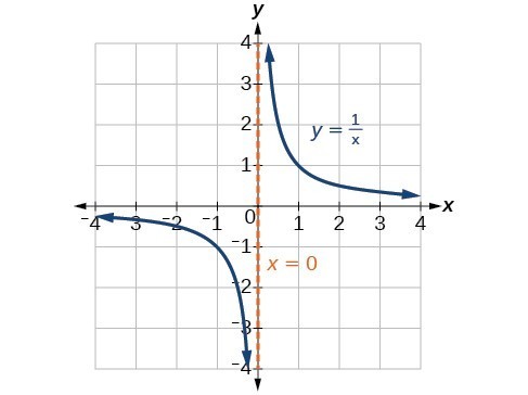
Figure 6
When the degree of the factor in the denominator is even, the distinguishing characteristic is that the graph either heads toward positive infinity on both sides of the vertical asymptote or heads toward negative infinity on both sides.
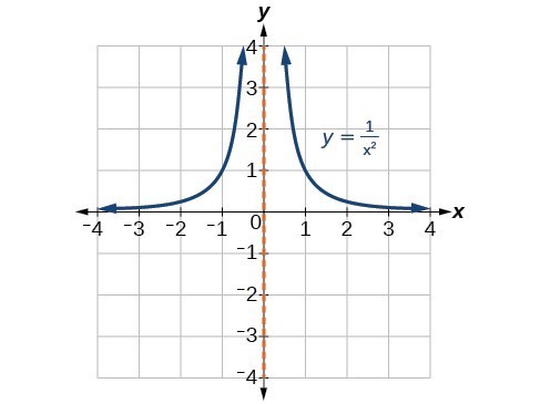
Figure 7
For example, the graph of [latex]f\left(x\right)=\frac{{\left(x+1\right)}^{2}\left(x - 3\right)}{{\left(x+3\right)}^{2}\left(x - 2\right)}[/latex] is shown in Figure 8.
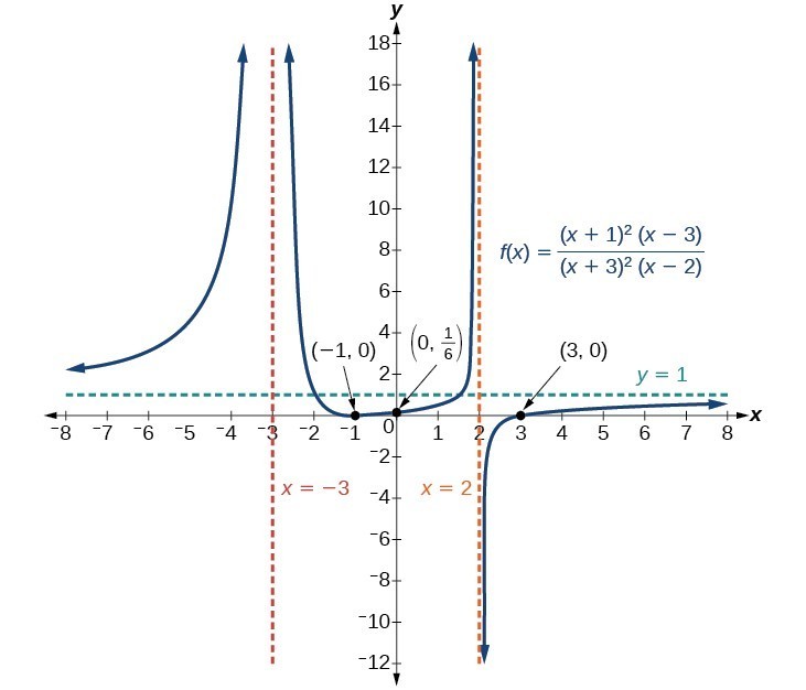
Figure 8
- At the x-intercept [latex]x=-1[/latex] corresponding to the [latex]{\left(x+1\right)}^{2}[/latex] factor of the numerator, the graph bounces, consistent with the quadratic nature of the factor.
- At the x-intercept [latex]x=3[/latex] corresponding to the [latex]\left(x - 3\right)[/latex] factor of the numerator, the graph passes through the axis as we would expect from a linear factor.
- At the vertical asymptote [latex]x=-3[/latex] corresponding to the [latex]{\left(x+3\right)}^{2}[/latex] factor of the denominator, the graph heads towards positive infinity on both sides of the asymptote, consistent with the behavior of the function [latex]f\left(x\right)=\frac{1}{{x}^{2}}[/latex].
- At the vertical asymptote [latex]x=2[/latex], corresponding to the [latex]\left(x - 2\right)[/latex] factor of the denominator, the graph heads towards positive infinity on the left side of the asymptote and towards negative infinity on the right side, consistent with the behavior of the function [latex]f\left(x\right)=\frac{1}{x}[/latex].
How To: Given a rational function, sketch a graph.
- Evaluate the function at 0 to find the y-intercept.
- Factor the numerator and denominator.
- For factors in the numerator not common to the denominator, determine where each factor of the numerator is zero to find the x-intercepts.
- Find the multiplicities of the x-intercepts to determine the behavior of the graph at those points.
- For factors in the denominator, note the multiplicities of the zeros to determine the local behavior. For those factors not common to the numerator, find the vertical asymptotes by setting those factors equal to zero and then solve.
- For factors in the denominator common to factors in the numerator, find the removable discontinuities by setting those factors equal to 0 and then solve.
- Compare the degrees of the numerator and the denominator to determine the horizontal or slant asymptotes.
- Sketch the graph.
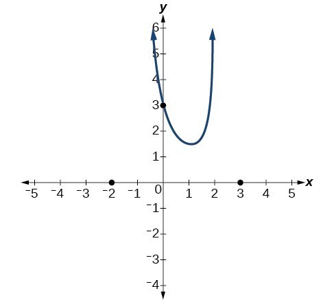
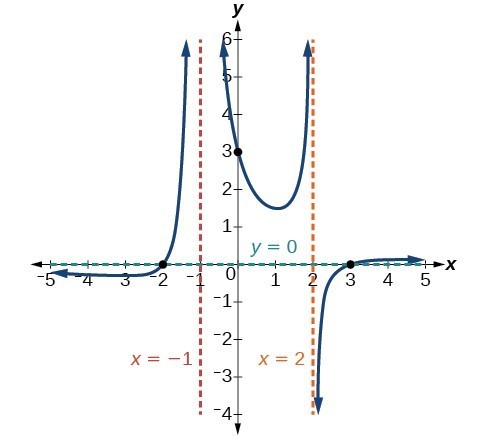
Example 3: Graphing a Rational Function
Sketch a graph of [latex]f\left(x\right)=\frac{\left(x+2\right)\left(x - 3\right)}{{\left(x+1\right)}^{2}\left(x - 2\right)}[/latex].
Try It
Given the function [latex]f\left(x\right)=\frac{{\left(x+2\right)}^{2}\left(x - 2\right)}{2{\left(x - 1\right)}^{2}\left(x - 3\right)}[/latex], use the characteristics of polynomials and rational functions to describe its behavior and sketch the function.

Try It
Key Equations
| Rational Function | [latex]f\left(x\right)=\dfrac{P\left(x\right)}{Q\left(x\right)}=\dfrac{{a}_{p}{x}^{p}+{a}_{p - 1}{x}^{p - 1}+...+{a}_{1}x+{a}_{0}}{{b}_{q}{x}^{q}+{b}_{q - 1}{x}^{q - 1}+...+{b}_{1}x+{b}_{0}}, Q\left(x\right)\ne 0[/latex] |
Key Concepts
- We can use arrow notation to describe local behavior and end behavior of the toolkit functions [latex]f\left(x\right)=\frac{1}{x}[/latex] and [latex]f\left(x\right)=\frac{1}{{x}^{2}}[/latex].
- Graph rational functions by finding the intercepts, behavior at the intercepts and asymptotes, and end behavior.
Glossary
- arrow notation
- a way to symbolically represent the local and end behavior of a function by using arrows to indicate that an input or output approaches a value
Section 4.4 Homework Exercises
For the following exercises, use the given transformation to graph the function. Note the vertical and horizontal asymptotes.
1. The reciprocal function shifted up two units.
2. The reciprocal function shifted down one unit and left three units.
3. The reciprocal squared function shifted to the right 2 units.
4. The reciprocal squared function shifted down 2 units and right 1 unit.
For the following exercises, find the horizontal intercepts, the vertical intercept, the vertical asymptotes, and the horizontal or slant asymptote of the functions. Use that information to sketch a graph.
5. [latex]p\left(x\right)=\frac{2x - 3}{x+4}[/latex]
6. [latex]q\left(x\right)=\frac{x - 5}{3x - 1}[/latex]
7. [latex]s\left(x\right)=\frac{4}{{\left(x - 2\right)}^{2}}[/latex]
8. [latex]r\left(x\right)=\frac{5}{{\left(x+1\right)}^{2}}[/latex]
9. [latex]f\left(x\right)=\frac{3{x}^{2}-14x - 5}{3{x}^{2}+8x - 16}[/latex]
10. [latex]g\left(x\right)=\frac{2{x}^{2}+7x - 15}{3{x}^{2}-14+15}[/latex]
11. [latex]a\left(x\right)=\frac{{x}^{2}+2x - 3}{{x}^{2}-1}[/latex]
12. [latex]b\left(x\right)=\frac{{x}^{2}-x - 6}{{x}^{2}-4}[/latex]
13. [latex]h\left(x\right)=\frac{2{x}^{2}+ x - 1}{x - 4}[/latex]
14. [latex]k\left(x\right)=\frac{2{x}^{2}-3x - 20}{x - 5}[/latex]
15. [latex]w\left(x\right)=\frac{\left(x - 1\right)\left(x+3\right)\left(x - 5\right)}{{\left(x+2\right)}^{2}\left(x - 4\right)}[/latex]
16. [latex]z\left(x\right)=\frac{{\left(x+2\right)}^{2}\left(x - 5\right)}{\left(x - 3\right)\left(x+1\right)\left(x+4\right)}[/latex]
For the following exercises, use a calculator to graph [latex]f\left(x\right)[/latex]. Use the graph to solve [latex]f\left(x\right)>0[/latex].
17. [latex]f\left(x\right)=\frac{4}{2x - 3}[/latex]
18. [latex]f\left(x\right)=\frac{2}{\left(x - 1\right)\left(x+2\right)}[/latex]
19. [latex]f\left(x\right)=\frac{x+2}{\left(x - 1\right)\left(x - 4\right)}[/latex]
20. [latex]f\left(x\right)=\frac{{\left(x+3\right)}^{2}}{{\left(x - 1\right)}^{2}\left(x+1\right)}[/latex]