Learning Objectives
- (11.2.1) – Graphing with transformations of functions
- Graph functions using vertical and horizontal shifts
- Graph functions using reflections about the [latex]x[/latex]-axis and the [latex]y[/latex]-axis
- Graph functions using compressions and stretches
- Combine transformations
- (11.2.2) – Transformations of quadratic functions
(11.2.1) – Graphing with transformations of functions
We all know that a flat mirror enables us to see an accurate image of ourselves and whatever is behind us. When we tilt the mirror, the images we see may shift horizontally or vertically. But what happens when we bend a flexible mirror? Like a carnival funhouse mirror, it presents us with a distorted image of ourselves, stretched or compressed horizontally or vertically. In a similar way, we can distort or transform mathematical functions to better adapt them to describing objects or processes in the real world. In this section, we will take a look at several kinds of transformations.

Figure 1. (credit: “Misko”/Flickr)
Graph functions using vertical and horizontal shifts
One simple kind of transformation involves shifting the entire graph of a function up, down, right, or left. The simplest shift is a vertical shift, moving the graph up or down, because this transformation involves adding a positive or negative constant to the function. In other words, we add the same constant to the output value of the function regardless of the input. For a function [latex]g\left(x\right)=f\left(x\right)+k[/latex], the function [latex]f\left(x\right)[/latex] is shifted vertically [latex]k[/latex] units.
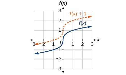
Vertical shift by [latex]k=1[/latex] of the cube root function [latex]f\left(x\right)=\sqrt[3]{x}[/latex].
To help you visualize the concept of a vertical shift, consider that [latex]y=f\left(x\right)[/latex]. Therefore, [latex]f\left(x\right)+k[/latex] is equivalent to [latex]y+k[/latex]. Every unit of [latex]y[/latex] is replaced by [latex]y+k[/latex], so the [latex]y\text{-}[/latex] value increases or decreases depending on the value of [latex]k[/latex]. The result is a shift upward or downward.
A General Note: Vertical Shift
Given a function [latex]f\left(x\right)[/latex], a new function [latex]g\left(x\right)=f\left(x\right)+k[/latex], where [latex]k[/latex] is a constant, is a vertical shift of the function [latex]f\left(x\right)[/latex]. All the output values change by [latex]k[/latex] units. If [latex]k[/latex] is positive, the graph will shift up. If [latex]k[/latex] is negative, the graph will shift down.
Example: Adding a Constant to a Function
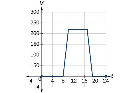
To regulate temperature in a green building, airflow vents near the roof open and close throughout the day. Figure 2 shows the area of open vents [latex]V[/latex] (in square feet) throughout the day in hours after midnight, [latex]t[/latex]. During the summer, the facilities manager decides to try to better regulate temperature by increasing the amount of open vents by 20 square feet throughout the day and night. Sketch a graph of this new function.

How To: Given a tabular function, create a new row to represent a vertical shift.
- Identify the output row or column.
- Determine the magnitude of the shift.
- Add the shift to the value in each output cell. Add a positive value for up or a negative value for down.
Example: Shifting a Tabular Function Vertically
A function [latex]f\left(x\right)[/latex] is given below. Create a table for the function [latex]g\left(x\right)=f\left(x\right)-3[/latex].
| [latex]x[/latex] | 2 | 4 | 6 | 8 |
| [latex]f\left(x\right)[/latex] | 1 | 3 | 7 | 11 |
Try It
The function [latex]h\left(t\right)=-4.9{t}^{2}+30t[/latex] gives the height [latex]h[/latex] of a ball (in meters) thrown upward from the ground after [latex]t[/latex] seconds. Suppose the ball was instead thrown from the top of a 10-m building. Relate this new height function [latex]b\left(t\right)[/latex] to [latex]h\left(t\right)[/latex], and then find a formula for [latex]b\left(t\right)[/latex].
Identifying Horizontal Shifts
We just saw that the vertical shift is a change to the output, or outside, of the function. We will now look at how changes to input, on the inside of the function, change its graph and meaning. A shift to the input results in a movement of the graph of the function left or right in what is known as a horizontal shift.
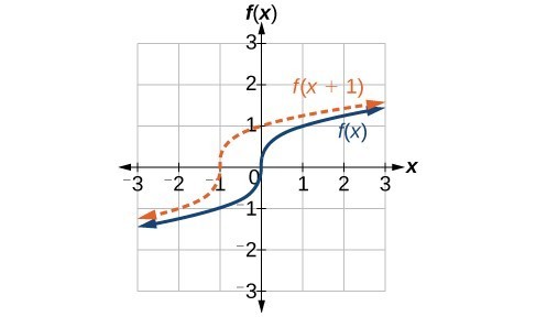
Horizontal shift of the function [latex]f\left(x\right)=\sqrt[3]{x}[/latex]. Note that [latex]h=+1[/latex] shifts the graph to the left, that is, towards negative values of [latex]x[/latex].
For example, if [latex]f\left(x\right)={x}^{2}[/latex], then [latex]g\left(x\right)={\left(x - 2\right)}^{2}[/latex] is a new function. Each input is reduced by 2 prior to squaring the function. The result is that the graph is shifted 2 units to the right, because we would need to increase the prior input by 2 units to yield the same output value as given in [latex]f[/latex].
A General Note: Horizontal Shift
Given a function [latex]f[/latex], a new function [latex]g\left(x\right)=f\left(x-h\right)[/latex], where [latex]h[/latex] is a constant, is a horizontal shift of the function [latex]f[/latex]. If [latex]h[/latex] is positive, the graph will shift right. If [latex]h[/latex] is negative, the graph will shift left.
Example: Adding a Constant to an Input
Returning to our building airflow example from Example 2, suppose that in autumn the facilities manager decides that the original venting plan starts too late, and wants to begin the entire venting program 2 hours earlier. Sketch a graph of the new function.

How To: Given a tabular function, create a new row to represent a horizontal shift.
- Identify the input row or column.
- Determine the magnitude of the shift.
- Add the shift to the value in each input cell.
Example: Shifting a Tabular Function Horizontally
A function [latex]f\left(x\right)[/latex] is given below. Create a table for the function [latex]g\left(x\right)=f\left(x - 3\right)[/latex].
| [latex]x[/latex] | 2 | 4 | 6 | 8 |
| [latex]f\left(x\right)[/latex] | 1 | 3 | 7 | 11 |

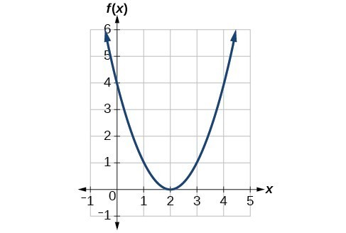
Example: Identifying a Horizontal Shift of a Toolkit Function
This graph represents a transformation of the toolkit function [latex]f\left(x\right)={x}^{2}[/latex]. Relate this new function [latex]g\left(x\right)[/latex] to [latex]f\left(x\right)[/latex], and then find a formula for [latex]g\left(x\right)[/latex].
Example: Interpreting Horizontal versus Vertical Shifts
The function [latex]G\left(m\right)[/latex] gives the number of gallons of gas required to drive [latex]m[/latex] miles. Interpret [latex]G\left(m\right)+10[/latex] and [latex]G\left(m+10\right)[/latex].
Try It
Given the function [latex]f\left(x\right)=\sqrt{x}[/latex], graph the original function [latex]f\left(x\right)[/latex] and the transformation [latex]g\left(x\right)=f\left(x+2\right)[/latex] on the same axes. Is this a horizontal or a vertical shift? Which way is the graph shifted and by how many units?
Graph functions using reflections about the [latex]x[/latex]-axis and the [latex]y[/latex]-axis
Another transformation that can be applied to a function is a reflection over the [latex]x[/latex]– or [latex]y[/latex]-axis. A vertical reflection reflects a graph vertically across the [latex]x[/latex]-axis, while a horizontal reflection reflects a graph horizontally across the [latex]y[/latex]-axis. The reflections are shown in Figure 9.
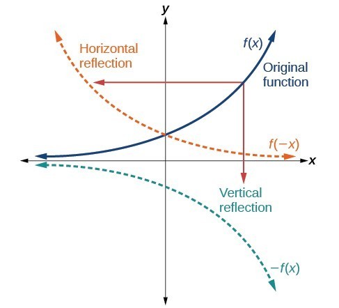
Vertical and horizontal reflections of a function.
Notice that the vertical reflection produces a new graph that is a mirror image of the base or original graph about the x-axis. The horizontal reflection produces a new graph that is a mirror image of the base or original graph about the y-axis.
A General Note: Reflections
Given a function [latex]f\left(x\right)[/latex], a new function [latex]g\left(x\right)=-f\left(x\right)[/latex] is a vertical reflection of the function [latex]f\left(x\right)[/latex], sometimes called a reflection about (or over, or through) the x-axis.
Given a function [latex]f\left(x\right)[/latex], a new function [latex]g\left(x\right)=f\left(-x\right)[/latex] is a horizontal reflection of the function [latex]f\left(x\right)[/latex], sometimes called a reflection about the y-axis.
How To: Given a function, reflect the graph both vertically and horizontally.
- Multiply all outputs by [latex]-1[/latex] for a vertical reflection. The new graph is a reflection of the original graph about the [latex]x[/latex]-axis.
- Multiply all inputs by [latex]-1[/latex] for a horizontal reflection. The new graph is a reflection of the original graph about the [latex]y[/latex]-axis.
Example: Reflecting a Graph Horizontally and Vertically
Reflect the graph of [latex]s\left(t\right)=\sqrt{t}[/latex] (a) vertically and (b) horizontally.


Try It
Reflect the graph of [latex]f\left(x\right)=|x - 1|[/latex] (a) vertically and (b) horizontally.


Example: Reflecting a Tabular Function Horizontally and Vertically
A function [latex]f\left(x\right)[/latex] is given. Create a table for the functions below.
- [latex]g\left(x\right)=-f\left(x\right)[/latex]
- [latex]h\left(x\right)=f\left(-x\right)[/latex]
| [latex]x[/latex] | 2 | 4 | 6 | 8 |
| [latex]f\left(x\right)[/latex] | 1 | 3 | 7 | 11 |
Try It
| [latex]x[/latex] | −2 | 0 | 2 | 4 |
| [latex]f\left(x\right)[/latex] | 5 | 10 | 15 | 20 |
Using the function [latex]f\left(x\right)[/latex] given in the table above, create a table for the functions below.
a. [latex]g\left(x\right)=-f\left(x\right)[/latex]
b. [latex]h\left(x\right)=f\left(-x\right)[/latex]
Graph functions using compressions and stretches
Adding a constant to the inputs or outputs of a function changed the position of a graph with respect to the axes, but it did not affect the shape of a graph. We now explore the effects of multiplying the inputs or outputs by some quantity.
We can transform the inside (input values) of a function or we can transform the outside (output values) of a function. Each change has a specific effect that can be seen graphically.
Vertical Stretches and Compressions
When we multiply a function by a positive constant, we get a function whose graph is stretched or compressed vertically in relation to the graph of the original function. If the constant is greater than 1, we get a vertical stretch; if the constant is between 0 and 1, we get a vertical compression. The graph below shows a function multiplied by constant factors 2 and 0.5 and the resulting vertical stretch and compression.
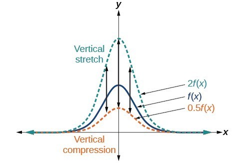
Vertical stretch and compression
A General Note: Vertical Stretches and Compressions
Given a function [latex]f\left(x\right)[/latex], a new function [latex]g\left(x\right)=af\left(x\right)[/latex], where [latex]a[/latex] is a constant, is a vertical stretch or vertical compression of the function [latex]f\left(x\right)[/latex].
- If [latex]a>1[/latex], then the graph will be stretched.
- If [latex]0 < a < 1[/latex], then the graph will be compressed.
- If [latex]a<0[/latex], then there will be combination of a vertical stretch or compression with a vertical reflection.
How To: Given a function, graph its vertical stretch.
- Identify the value of [latex]a[/latex].
- Multiply all range values by [latex]a[/latex].
- If [latex]a>1[/latex], the graph is stretched by a factor of [latex]a[/latex].
If [latex]{ 0 }<{ a }<{ 1 }[/latex], the graph is compressed by a factor of [latex]a[/latex]. If [latex]a<0[/latex], the graph is either stretched or compressed and also reflected about the x-axis.
Example: Graphing a Vertical Stretch
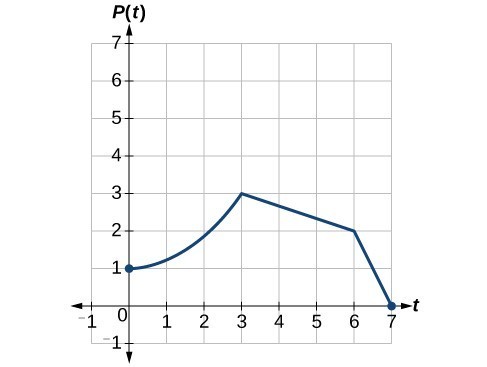
A function [latex]P\left(t\right)[/latex] models the number of fruit flies in a population over time, and is graphed below.
A scientist is comparing this population to another population, [latex]Q[/latex], whose growth follows the same pattern, but is twice as large. Sketch a graph of this population.

How To: Given a tabular function and assuming that the transformation is a vertical stretch or compression, create a table for a vertical compression.
- Determine the value of [latex]a[/latex].
- Multiply all of the output values by [latex]a[/latex].
Example: Finding a Vertical Compression of a Tabular Function
A function [latex]f[/latex] is given in the table below. Create a table for the function [latex]g\left(x\right)=\frac{1}{2}f\left(x\right)[/latex].
| [latex]x[/latex] | 2 | 4 | 6 | 8 |
| [latex]f\left(x\right)[/latex] | 1 | 3 | 7 | 11 |
EXAMPLE
A function [latex]f[/latex] is given below. Create a table for the function [latex]g\left(x\right)=\frac{3}{4}f\left(x\right)[/latex].
| [latex]x[/latex] | 2 | 4 | 6 | 8 |
| [latex]f\left(x\right)[/latex] | 12 | 16 | 20 | 0 |
Example: Recognizing a Vertical Stretch
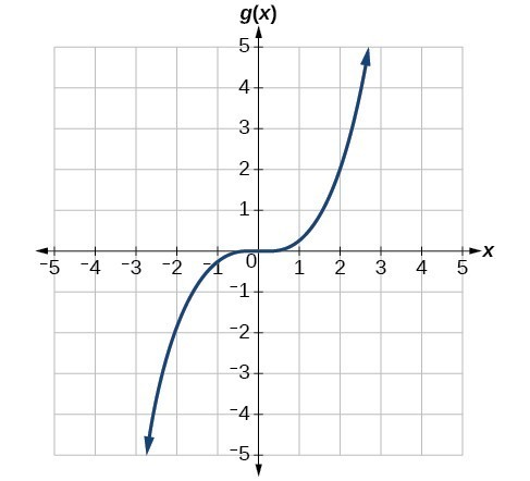
The graph is a transformation of the toolkit function [latex]f\left(x\right)={x}^{3}[/latex]. Relate this new function [latex]g\left(x\right)[/latex] to [latex]f\left(x\right)[/latex], and then find a formula for [latex]g\left(x\right)[/latex].
EXAMPLE
Write the formula for the function that we get when we stretch the identity toolkit function by a factor of 3, and then shift it down by 2 units.
Horizontal Stretches and Compressions
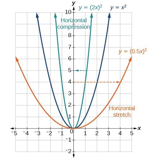
Now we consider changes to the inside of a function. When we multiply a function’s input by a positive constant, we get a function whose graph is stretched or compressed horizontally in relation to the graph of the original function. If the constant is between 0 and 1, we get a horizontal stretch; if the constant is greater than 1, we get a horizontal compression of the function.
Given a function [latex]y=f\left(x\right)[/latex], the form [latex]y=f\left(bx\right)[/latex] results in a horizontal stretch or compression. Consider the function [latex]y={x}^{2}[/latex]. The graph of [latex]y={\left(0.5x\right)}^{2}[/latex] is a horizontal stretch of the graph of the function [latex]y={x}^{2}[/latex] by a factor of 2. The graph of [latex]y={\left(2x\right)}^{2}[/latex] is a horizontal compression of the graph of the function [latex]y={x}^{2}[/latex] by a factor of 2.
A General Note: Horizontal Stretches and Compressions
Given a function [latex]f\left(x\right)[/latex], a new function [latex]g\left(x\right)=f\left(bx\right)[/latex], where [latex]b[/latex] is a constant, is a horizontal stretch or horizontal compression of the function [latex]f\left(x\right)[/latex].
- If [latex]b>1[/latex], then the graph will be compressed by [latex]\displaystyle \frac{1}{b}[/latex].
- If [latex]0
- If [latex]b<0[/latex], then there will be combination of a horizontal stretch or compression with a horizontal reflection.
How To: Given a description of a function, sketch a horizontal compression or stretch.
- Write a formula to represent the function.
- Set [latex]g\left(x\right)=f\left(bx\right)[/latex] where [latex]b>1[/latex] for a compression or [latex]0
Example: Graphing a Horizontal Compression
Suppose a scientist is comparing a population of fruit flies to a population that progresses through its lifespan twice as fast as the original population. In other words, this new population, [latex]R[/latex], will progress in 1 hour the same amount as the original population does in 2 hours, and in 2 hours, it will progress as much as the original population does in 4 hours. Sketch a graph of this population.
![Two side-by-side graphs. The first graph has function for original population whose domain is [0,7] and range is [0,3]. The maximum value occurs at (3,3). The second graph has the same shape as the first except it is half as wide. It is a graph of transformed population, with a domain of [0, 3.5] and a range of [0,3]. The maximum occurs at (1.5, 3).](https://s3-us-west-2.amazonaws.com/courses-images/wp-content/uploads/sites/2862/2017/12/26165351/CNX_Precalc_Figure_01_05_029ab.jpg)
Example: Finding a Horizontal Stretch for a Tabular Function
A function [latex]f\left(x\right)[/latex] is given below. Create a table for the function [latex]\displaystyle g\left(x\right)=f\left(\frac{1}{2}x\right)[/latex].
| [latex]x[/latex] | 2 | 4 | 6 | 8 |
| [latex]f\left(x\right)[/latex] | 1 | 3 | 7 | 11 |

Example: Recognizing a Horizontal Compression on a Graph
Relate the function [latex]g\left(x\right)[/latex] to [latex]f\left(x\right)[/latex].
Try It
Write a formula for the toolkit square root function horizontally stretched by a factor of 3.
Combine transformations
Now that we have two transformations, we can combine them together. Vertical shifts are outside changes that affect the output ( [latex]y\text{-}[/latex] ) axis values and shift the function up or down. Horizontal shifts are inside changes that affect the input ( [latex]x\text{-}[/latex] ) axis values and shift the function left or right. Combining the two types of shifts will cause the graph of a function to shift up or down and right or left.
How To: Given a function and both a vertical and a horizontal shift, sketch the graph.
- Identify the vertical and horizontal shifts from the formula.
- The vertical shift results from a constant added to the output. Move the graph up for a positive constant and down for a negative constant.
- The horizontal shift results from a constant added to the input. Move the graph left for a positive constant and right for a negative constant.
- Apply the shifts to the graph in either order.
Example: Graphing Combined Vertical and Horizontal Shifts
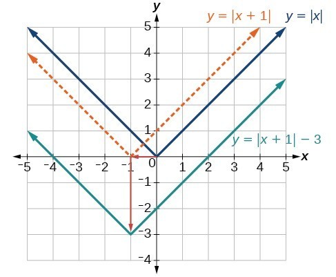
Given [latex]f\left(x\right)=|x|[/latex], sketch a graph of [latex]h\left(x\right)=f\left(x+1\right)-3[/latex].
The function [latex]f[/latex] is our toolkit absolute value function. We know that this graph has a V shape, with the point at the origin. The graph of [latex]h[/latex] has transformed [latex]f[/latex] in two ways: [latex]f\left(x+1\right)[/latex] is a change on the inside of the function, giving a horizontal shift left by 1, and the subtraction by 3 in [latex]f\left(x+1\right)-3[/latex] is a change to the outside of the function, giving a vertical shift down by 3. The transformation of the graph is illustrated below.
Let us follow one point of the graph of [latex]f\left(x\right)=|x|[/latex].
- The point [latex]\left(0,0\right)[/latex] is transformed first by shifting left 1 unit: [latex]\left(0,0\right)\to \left(-1,0\right)[/latex]
- The point [latex]\left(-1,0\right)[/latex] is transformed next by shifting down 3 units: [latex]\left(-1,0\right)\to \left(-1,-3\right)[/latex]
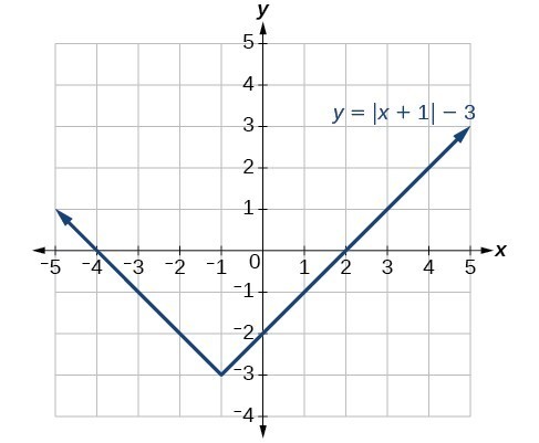
Below is the graph of [latex]h[/latex].
Try It
Given [latex]f\left(x\right)=|x|[/latex], sketch a graph of [latex]h\left(x\right)=f\left(x - 2\right)+4[/latex].

Example: Identifying Combined Vertical and Horizontal Shifts
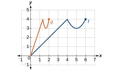
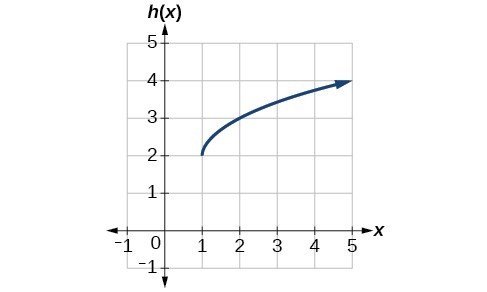
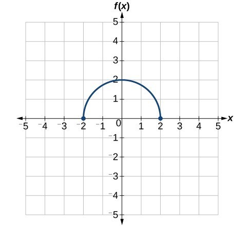
Write a formula for the graph shown below, which is a transformation of the toolkit square root function.
EXAMPLE
Write a formula for a transformation of the toolkit reciprocal function [latex]\displaystyle f\left(x\right)=\frac{1}{x}[/latex] that shifts the function’s graph one unit to the right and one unit up.
EXAMPLE
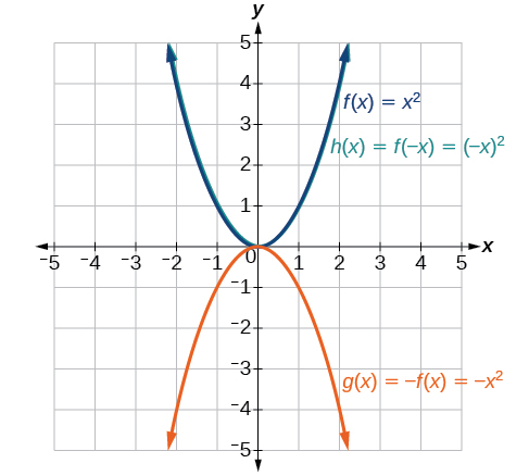
Given the toolkit function [latex]f\left(x\right)={x}^{2}[/latex], graph [latex]g\left(x\right)=-f\left(x\right)[/latex] and [latex]h\left(x\right)=f\left(-x\right)[/latex]. Take note of any surprising behavior for these functions.
Combine Shifts and Stretches
When combining transformations, it is very important to consider the order of the transformations. For example, vertically shifting by 3 and then vertically stretching by 2 does not create the same graph as vertically stretching by 2 and then vertically shifting by 3, because when we shift first, both the original function and the shift get stretched, while only the original function gets stretched when we stretch first.
When we see an expression such as [latex]2f\left(x\right)+3[/latex], which transformation should we start with? The answer here follows nicely from the order of operations. Given the output value of [latex]f\left(x\right)[/latex], we first multiply by 2, causing the vertical stretch, and then add 3, causing the vertical shift. In other words, multiplication before addition.
Horizontal transformations are a little trickier to think about. When we write [latex]g\left(x\right)=f\left(2x+3\right)[/latex], for example, we have to think about how the inputs to the function [latex]g[/latex] relate to the inputs to the function [latex]f[/latex]. Suppose we know [latex]f\left(7\right)=12[/latex]. What input to [latex]g[/latex] would produce that output? In other words, what value of [latex]x[/latex] will allow [latex]g\left(x\right)=f\left(2x+3\right)=12[/latex]? We would need [latex]2x+3=7[/latex]. To solve for [latex]x[/latex], we would first subtract 3, resulting in a horizontal shift, and then divide by 2, causing a horizontal compression.
This format ends up being very difficult to work with, because it is usually much easier to horizontally stretch a graph before shifting. We can work around this by factoring inside the function.
[latex]\displaystyle f\left(bx+p\right)=f\left(b\left(x+\frac{p}{b}\right)\right)[/latex]
Let’s work through an example.
[latex]f\left(x\right)={\left(2x+4\right)}^{2}[/latex]
We can factor out a 2.
[latex]f\left(x\right)={\left(2\left(x+2\right)\right)}^{2}[/latex]
Now we can more clearly observe a horizontal shift to the left 2 units and a horizontal compression. Factoring in this way allows us to horizontally stretch first and then shift horizontally.
A General Note: Combining Transformations
When combining vertical transformations written in the form [latex]af\left(x\right)+k[/latex], first vertically stretch by [latex]a[/latex] and then vertically shift by [latex]k[/latex].
When combining horizontal transformations written in the form [latex]f\left(bx+h\right)[/latex], first horizontally shift by [latex]h[/latex] and then horizontally stretch by [latex]\displaystyle \frac{1}{b}[/latex].
When combining horizontal transformations written in the form [latex]f\left(b\left(x+h\right)\right)[/latex], first horizontally stretch by [latex]\displaystyle \frac{1}{b}[/latex] and then horizontally shift by [latex]h[/latex].
Horizontal and vertical transformations are independent. It does not matter whether horizontal or vertical transformations are performed first.
Example: Finding a Triple Transformation of a Tabular Function
Given the table below for the function [latex]f\left(x\right)[/latex], create a table of values for the function [latex]g\left(x\right)=2f\left(3x\right)+1[/latex].
| [latex]x[/latex] | 6 | 12 | 18 | 24 |
| [latex]f\left(x\right)[/latex] | 10 | 14 | 15 | 17 |
Example: Finding a Triple Transformation of a Graph
Use the graph of [latex]f\left(x\right)[/latex] to sketch a graph of [latex]\displaystyle k\left(x\right)=f\left(\frac{1}{2}x+1\right)-3[/latex].


(11.2.2) – Transformations of Quadratic Functions
The standard form of a quadratic function presents the function in the form
where [latex]\left(h,\text{ }k\right)[/latex] is the vertex. Because the vertex appears in the standard form of the quadratic function, this form is also known as the vertex form of a quadratic function.
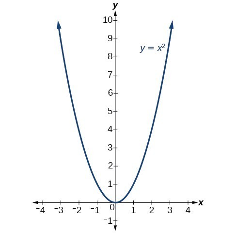
The standard form is useful for determining how the graph is transformed from the graph of [latex]y={x}^{2}[/latex]. The figure below is the graph of this basic function.
Shift Up and Down by Changing the value of [latex]k[/latex]
You can represent a vertical (up, down) shift of the graph of [latex]f(x)=x^2[/latex] by adding or subtracting a constant, [latex]k[/latex].
[latex]f(x)=x^2 + k[/latex]
If [latex]k>0[/latex], the graph shifts upward, whereas if [latex]k<0[/latex], the graph shifts downward.
Make Note
Write the equation for the graph of [latex]f(x)=x^2[/latex] that has been shifted up 4 units in the textbox below.
Now write the equation for the graph of [latex]f(x)=x^2[/latex] that has been shifted down 4 units in the textbox below.
Now check yourself!
Shift left and right by changing the value of [latex]h[/latex].
You can represent a horizontal (left, right) shift of the graph of [latex]f(x)=x^2[/latex] by adding or subtracting a constant, [latex]h[/latex], to the variable [latex]x[/latex], before squaring.
[latex]f(x)=(x-h)^2[/latex]
If [latex]h>0[/latex], the graph shifts toward the right and if [latex]h<0[/latex], the graph shifts to the left.
Make Note
Write the equation for the graph of [latex]f(x)=x^2[/latex] that has been shifted right 2 units in the textbox below.
Now write the equation for the graph of [latex]f(x)=x^2[/latex] that has been shifted left 2 units in the textbox below.
Now check yourself!
Stretch or compress by changing the value of [latex]a[/latex].
You can represent a stretch or compression (narrowing, widening) of the graph of [latex]f(x)=x^2[/latex] by multiplying the squared variable by a constant, a.
[latex]f(x)=ax^2[/latex]
The magnitude of a indicates the stretch of the graph. If [latex]|a|>1[/latex], the point associated with a particular x-value shifts farther from the x-axis, so the graph appears to become narrower, and there is a vertical stretch. But if [latex]|a|<1[/latex], the point associated with a particular x-value shifts closer to the x-axis, so the graph appears to become wider, but in fact there is a vertical compression.
Make Note
Write the equation for the graph of [latex]f(x)=x^2[/latex] that has been has been compressed vertically by a factor of [latex]\displaystyle \frac{1}{2}[/latex] in the textbox below.
Then, write the equation for the graph of [latex]f(x)=x^2[/latex] that has been vertically stretched by a factor of 3.
Now check yourself!
The standard form and the general form are equivalent methods of describing the same function. We can see this by expanding out the general form and setting it equal to the standard form.
For the linear terms to be equal, the coefficients must be equal.
This is the axis of symmetry we defined earlier. Setting the constant terms equal:
In practice, though, it is usually easier to remember that [latex]k[/latex] is the output value of the function when the input is [latex]h[/latex], so [latex]f\left(h\right)=k[/latex].
Summary of Transformations
| Vertical shift | [latex]g\left(x\right)=f\left(x\right)+k[/latex] (up for [latex]k>0[/latex] ) |
| Horizontal shift | [latex]g\left(x\right)=f\left(x-h\right)[/latex] (right for [latex]h>0[/latex] ) |
| Vertical reflection | [latex]g\left(x\right)=-f\left(x\right)[/latex] |
| Horizontal reflection | [latex]g\left(x\right)=f\left(-x\right)[/latex] |
| Vertical stretch | [latex]g\left(x\right)=af\left(x\right)[/latex] ( [latex]a>0[/latex]) |
| Vertical compression | [latex]g\left(x\right)=af\left(x\right)[/latex] [latex]\left(0 |
| Horizontal stretch | [latex]g\left(x\right)=f\left(bx\right)[/latex] [latex]\left(0 |
| Horizontal compression | [latex]g\left(x\right)=f\left(bx\right)[/latex] ( [latex]b>1[/latex] ) |
Candela Citations
- Revision and Adaptation. Provided by: Lumen Learning. License: CC BY: Attribution
- Question ID 113437, 60789, 112701, 60650, 113454, 112703, 112707, 112726, 113225. Authored by: Lumen Learning. License: CC BY: Attribution. License Terms: IMathAS Community License CC-BY + GPL
- Interactive: Transform Quadratic 1. Provided by: Lumen Learning (with Desmos). Located at: https://www.desmos.com/calculator/fpatj6tbcn. License: CC BY: Attribution
- Interactive: Transform Quadratic 2. Provided by: Lumen Learning (with Desmos). License: CC BY: Attribution
- Interactive: Transform Quadratic 3. Provided by: Lumen Learning (with Desmos). Located at: https://www.desmos.com/calculator/ha6gh59rq7. License: CC BY: Attribution
- Interactive: Transform Quadratic 4. Provided by: Lumen Learning (with Desmos). Located at: https://www.desmos.com/calculator/pimelalx4i. License: CC BY: Attribution
- College Algebra. Authored by: Abramson, Jay et al.. Provided by: OpenStax. Located at: http://cnx.org/contents/9b08c294-057f-4201-9f48-5d6ad992740d@5.2. License: CC BY: Attribution. License Terms: Download for free at http://cnx.org/contents/9b08c294-057f-4201-9f48-5d6ad992740d@5.2
- Question ID 75586, 75929, 75931. Authored by: Shahbazian, Roy. License: CC BY: Attribution. License Terms: IMathAS Community License CC-BY + GPL
- Question ID 33066. Authored by: Smart, Jim. License: CC BY: Attribution. License Terms: IMathAS Community License CC-BY + GPL
- Question ID 74696, 74730. Authored by: Meacham, William. License: CC BY: Attribution. License Terms: IMathAS Community License CC-BY + GPL
- Question ID 60791, 60790. Authored by: Day, Alyson. License: CC BY: Attribution. License Terms: IMathAS Community License CC-BY + GPL