Adding a constant to the inputs or outputs of a function changed the position of a graph with respect to the axes, but it did not affect the shape of a graph. We now explore the effects of multiplying the inputs or outputs by some quantity.
We can transform the inside (input values) of a function or we can transform the outside (output values) of a function. Each change has a specific effect that can be seen graphically.
Vertical Stretches and Compressions
When we multiply a function by a positive constant, we get a function whose graph is stretched or compressed vertically in relation to the graph of the original function. If the constant is greater than 1, we get a vertical stretch; if the constant is between 0 and 1, we get a vertical compression. The graph below shows a function multiplied by constant factors 2 and 0.5 and the resulting vertical stretch and compression.
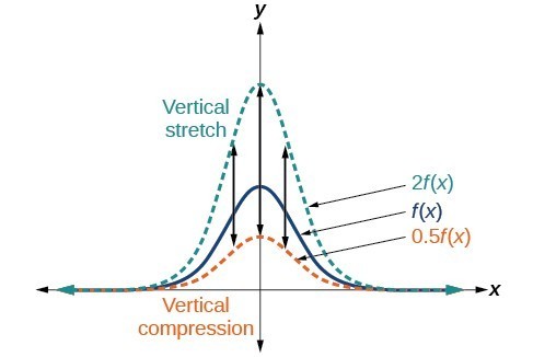
Figure 14. Vertical stretch and compression
A General Note: Vertical Stretches and Compressions
Given a function [latex]f\left(x\right)[/latex], a new function [latex]g\left(x\right)=af\left(x\right)[/latex], where [latex]a[/latex] is a constant, is a vertical stretch or vertical compression of the function [latex]f\left(x\right)[/latex].
- If [latex]a>1[/latex], then the graph will be stretched.
- If 0 < a < 1, then the graph will be compressed.
- If [latex]a<0[/latex], then there will be combination of a vertical stretch or compression with a vertical reflection.
How To: Given a function, graph its vertical stretch.
- Identify the value of [latex]a[/latex].
- Multiply all range values by [latex]a[/latex].
-
If [latex]a>1[/latex], the graph is stretched by a factor of [latex]a[/latex].
If [latex]{ 0 }<{ a }<{ 1 }[/latex], the graph is compressed by a factor of [latex]a[/latex].
If [latex]a<0[/latex], the graph is either stretched or compressed and also reflected about the x-axis.
Example 10: Graphing a Vertical Stretch
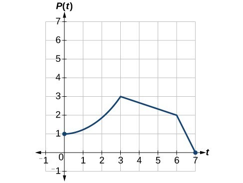
Figure 15
A function [latex]P\left(t\right)[/latex] models the population of fruit flies.
A scientist is comparing this population to another population, [latex]Q[/latex], whose growth follows the same pattern, but is twice as large. Sketch a graph of this population.
Solution
Because the population is always twice as large, the new population’s output values are always twice the original function’s output values.
If we choose four reference points, (0, 1), (3, 3), (6, 2) and (7, 0) we will multiply all of the outputs by 2.
The following shows where the new points for the new graph will be located.
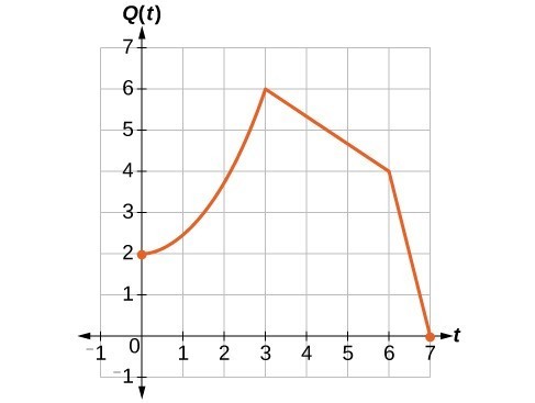
Figure 16
Symbolically, the relationship is written as
This means that for any input [latex]t[/latex], the value of the function [latex]Q[/latex] is twice the value of the function [latex]P[/latex]. Notice that the effect on the graph is a vertical stretching of the graph, where every point doubles its distance from the horizontal axis. The input values, [latex]t[/latex], stay the same while the output values are twice as large as before.
How To: Given a tabular function and assuming that the transformation is a vertical stretch or compression, create a table for a vertical compression.
- Determine the value of [latex]a[/latex].
- Multiply all of the output values by [latex]a[/latex].
Example 11: Finding a Vertical Compression of a Tabular Function
A function [latex]f[/latex] is given in the table below. Create a table for the function [latex]g\left(x\right)=\frac{1}{2}f\left(x\right)[/latex].
| [latex]x[/latex] | 2 | 4 | 6 | 8 |
| [latex]f\left(x\right)[/latex] | 1 | 3 | 7 | 11 |
Solution
The formula [latex]g\left(x\right)=\frac{1}{2}f\left(x\right)[/latex] tells us that the output values of [latex]g[/latex] are half of the output values of [latex]f[/latex] with the same inputs. For example, we know that [latex]f\left(4\right)=3[/latex]. Then
We do the same for the other values to produce this table.
| [latex]x[/latex] | [latex]2[/latex] | [latex]4[/latex] | [latex]6[/latex] | [latex]8[/latex] |
| [latex]g\left(x\right)[/latex] | [latex]\frac{1}{2}[/latex] | [latex]\frac{3}{2}[/latex] | [latex]\frac{7}{2}[/latex] | [latex]\frac{11}{2}[/latex] |
Try It 5
A function [latex]f[/latex] is given below. Create a table for the function [latex]g\left(x\right)=\frac{3}{4}f\left(x\right)[/latex].
| [latex]x[/latex] | 2 | 4 | 6 | 8 |
| [latex]f\left(x\right)[/latex] | 12 | 16 | 20 | 0 |
Example 12: Recognizing a Vertical Stretch
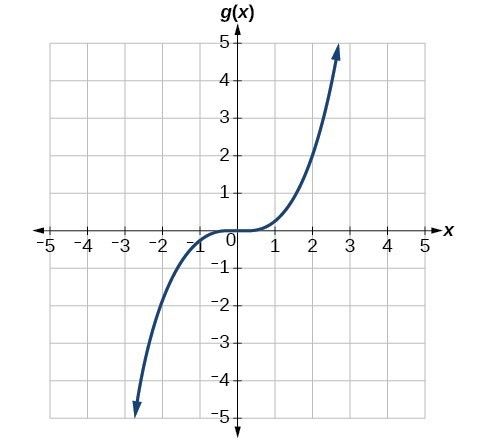
Figure 17
The graph is a transformation of the toolkit function [latex]f\left(x\right)={x}^{3}[/latex]. Relate this new function [latex]g\left(x\right)[/latex] to [latex]f\left(x\right)[/latex], and then find a formula for [latex]g\left(x\right)[/latex].
Solution
When trying to determine a vertical stretch or shift, it is helpful to look for a point on the graph that is relatively clear. In this graph, it appears that [latex]g\left(2\right)=2[/latex]. With the basic cubic function at the same input, [latex]f\left(2\right)={2}^{3}=8[/latex]. Based on that, it appears that the outputs of [latex]g[/latex] are [latex]\frac{1}{4}[/latex] the outputs of the function [latex]f[/latex] because [latex]g\left(2\right)=\frac{1}{4}f\left(2\right)[/latex]. From this we can fairly safely conclude that [latex]g\left(x\right)=\frac{1}{4}f\left(x\right)[/latex].
We can write a formula for [latex]g[/latex] by using the definition of the function [latex]f[/latex].
Try It 6
Write the formula for the function that we get when we stretch the identity toolkit function by a factor of 3, and then shift it down by 2 units.
Horizontal Stretches and Compressions
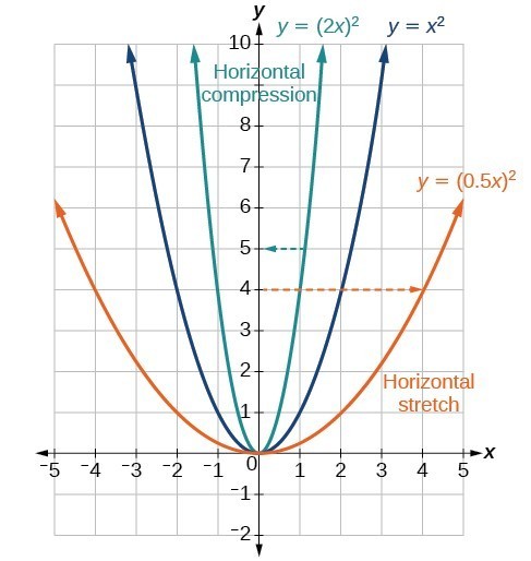
Figure 18
Now we consider changes to the inside of a function. When we multiply a function’s input by a positive constant, we get a function whose graph is stretched or compressed horizontally in relation to the graph of the original function. If the constant is between 0 and 1, we get a horizontal stretch; if the constant is greater than 1, we get a horizontal compression of the function.
Given a function [latex]y=f\left(x\right)[/latex], the form [latex]y=f\left(bx\right)[/latex] results in a horizontal stretch or compression. Consider the function [latex]y={x}^{2}[/latex]. The graph of [latex]y={\left(0.5x\right)}^{2}[/latex] is a horizontal stretch of the graph of the function [latex]y={x}^{2}[/latex] by a factor of 2. The graph of [latex]y={\left(2x\right)}^{2}[/latex] is a horizontal compression of the graph of the function [latex]y={x}^{2}[/latex] by a factor of 2.
A General Note: Horizontal Stretches and Compressions
Given a function [latex]f\left(x\right)[/latex], a new function [latex]g\left(x\right)=f\left(bx\right)[/latex], where [latex]b[/latex] is a constant, is a horizontal stretch or horizontal compression of the function [latex]f\left(x\right)[/latex].
- If [latex]b>1[/latex], then the graph will be compressed by [latex]\frac{1}{b}[/latex].
- If [latex]0
- If [latex]b<0[/latex], then there will be combination of a horizontal stretch or compression with a horizontal reflection.
How To: Given a description of a function, sketch a horizontal compression or stretch.
- Write a formula to represent the function.
- Set [latex]g\left(x\right)=f\left(bx\right)[/latex] where [latex]b>1[/latex] for a compression or [latex]0
Example 13: Graphing a Horizontal Compression
Suppose a scientist is comparing a population of fruit flies to a population that progresses through its lifespan twice as fast as the original population. In other words, this new population, [latex]R[/latex], will progress in 1 hour the same amount as the original population does in 2 hours, and in 2 hours, it will progress as much as the original population does in 4 hours. Sketch a graph of this population.
Solution
Symbolically, we could write
See below for a graphical comparison of the original population and the compressed population.
![Two side-by-side graphs. The first graph has function for original population whose domain is [0,7] and range is [0,3]. The maximum value occurs at (3,3). The second graph has the same shape as the first except it is half as wide. It is a graph of transformed population, with a domain of [0, 3.5] and a range of [0,3]. The maximum occurs at (1.5, 3).](https://s3-us-west-2.amazonaws.com/courses-images-archive-read-only/wp-content/uploads/sites/924/2015/11/25200820/CNX_Precalc_Figure_01_05_029ab.jpg)
Figure 19. (a) Original population graph (b) Compressed population graph
Analysis of the Solution
Note that the effect on the graph is a horizontal compression where all input values are half of their original distance from the vertical axis.
Example 14: Finding a Horizontal Stretch for a Tabular Function
A function [latex]f\left(x\right)[/latex] is given below. Create a table for the function [latex]g\left(x\right)=f\left(\frac{1}{2}x\right)[/latex].
| [latex]x[/latex] | 2 | 4 | 6 | 8 |
| [latex]f\left(x\right)[/latex] | 1 | 3 | 7 | 11 |
Solution
The formula [latex]g\left(x\right)=f\left(\frac{1}{2}x\right)[/latex] tells us that the output values for [latex]g[/latex] are the same as the output values for the function [latex]f[/latex] at an input half the size. Notice that we do not have enough information to determine [latex]g\left(2\right)[/latex] because [latex]g\left(2\right)=f\left(\frac{1}{2}\cdot 2\right)=f\left(1\right)[/latex], and we do not have a value for [latex]f\left(1\right)[/latex] in our table. Our input values to [latex]g[/latex] will need to be twice as large to get inputs for [latex]f[/latex] that we can evaluate. For example, we can determine [latex]g\left(4\right)\text{.}[/latex]
We do the same for the other values to produce the table below.
| [latex]x[/latex] | 4 | 8 | 12 | 16 |
| [latex]g\left(x\right)[/latex] | 1 | 3 | 7 | 11 |
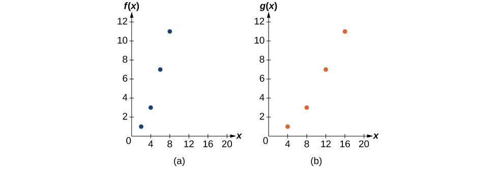
Figure 20
This figure shows the graphs of both of these sets of points.
Analysis of the Solution
Because each input value has been doubled, the result is that the function [latex]g\left(x\right)[/latex] has been stretched horizontally by a factor of 2.
Example 15: Recognizing a Horizontal Compression on a Graph
Relate the function [latex]g\left(x\right)[/latex] to [latex]f\left(x\right)[/latex] in Figure 21.
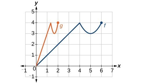
Figure 21
Solution
The graph of [latex]g\left(x\right)[/latex] looks like the graph of [latex]f\left(x\right)[/latex] horizontally compressed. Because [latex]f\left(x\right)[/latex] ends at [latex]\left(6,4\right)[/latex] and [latex]g\left(x\right)[/latex] ends at [latex]\left(2,4\right)[/latex], we can see that the [latex]x\text{-}[/latex] values have been compressed by [latex]\frac{1}{3}[/latex], because [latex]6\left(\frac{1}{3}\right)=2[/latex]. We might also notice that [latex]g\left(2\right)=f\left(6\right)[/latex] and [latex]g\left(1\right)=f\left(3\right)[/latex]. Either way, we can describe this relationship as [latex]g\left(x\right)=f\left(3x\right)[/latex]. This is a horizontal compression by [latex]\frac{1}{3}[/latex].
Analysis of the Solution
Notice that the coefficient needed for a horizontal stretch or compression is the reciprocal of the stretch or compression. So to stretch the graph horizontally by a scale factor of 4, we need a coefficient of [latex]\frac{1}{4}[/latex] in our function: [latex]f\left(\frac{1}{4}x\right)[/latex]. This means that the input values must be four times larger to produce the same result, requiring the input to be larger, causing the horizontal stretching.
Try It 7
Write a formula for the toolkit square root function horizontally stretched by a factor of 3.
Candela Citations
- Precalculus. Authored by: Jay Abramson, et al.. Provided by: OpenStax. Located at: http://cnx.org/contents/fd53eae1-fa23-47c7-bb1b-972349835c3c@5.175. License: CC BY: Attribution. License Terms: Download For Free at : http://cnx.org/contents/fd53eae1-fa23-47c7-bb1b-972349835c3c@5.175.
Analysis of the Solution
The result is that the function [latex]g\left(x\right)[/latex] has been compressed vertically by [latex]\frac{1}{2}[/latex]. Each output value is divided in half, so the graph is half the original height.