We can use what we have learned about multiplicities, end behavior, and turning points to sketch graphs of polynomial functions. Let us put this all together and look at the steps required to graph polynomial functions.
How To: Given a polynomial function, sketch the graph.
- Find the intercepts.
- Check for symmetry. If the function is an even function, its graph is symmetrical about the y-axis, that is, f(–x) = f(x).
If a function is an odd function, its graph is symmetrical about the origin, that is, f(–x) = –f(x). - Use the multiplicities of the zeros to determine the behavior of the polynomial at the x-intercepts.
- Determine the end behavior by examining the leading term.
- Use the end behavior and the behavior at the intercepts to sketch a graph.
- Ensure that the number of turning points does not exceed one less than the degree of the polynomial.
- Optionally, use technology to check the graph.
Example 8: Sketching the Graph of a Polynomial Function
Sketch a graph of [latex]f\left(x\right)=-2{\left(x+3\right)}^{2}\left(x - 5\right)[/latex].
Solution
This graph has two x-intercepts. At x = –3, the factor is squared, indicating a multiplicity of 2. The graph will bounce at this x-intercept. At x = 5, the function has a multiplicity of one, indicating the graph will cross through the axis at this intercept.
The y-intercept is found by evaluating f(0).
The y-intercept is (0, 90).
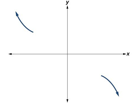
Figure 13
Additionally, we can see the leading term, if this polynomial were multiplied out, would be [latex]-2{x}^{3}[/latex],
so the end behavior is that of a vertically reflected cubic, with the outputs decreasing as the inputs approach infinity, and the outputs increasing as the inputs approach negative infinity.
To sketch this, we consider that:
- As [latex]x\to -\infty[/latex] the function [latex]f\left(x\right)\to \infty[/latex], so we know the graph starts in the second quadrant and is decreasing toward the x-axis.
- Since [latex]f\left(-x\right)=-2{\left(-x+3\right)}^{2}\left(-x - 5\right)[/latex]
is not equal to f(x), the graph does not display symmetry. - At [latex]\left(-3,0\right)[/latex], the graph bounces off of the x-axis, so the function must start increasing.
At (0, 90), the graph crosses the y-axis at the y-intercept.

Figure 14
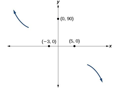
Figure 15
Somewhere after this point, the graph must turn back down or start decreasing toward the horizontal axis because the graph passes through the next intercept at (5, 0).
As [latex]x\to \infty[/latex] the function [latex]f\left(x\right)\to \mathrm{-\infty }[/latex], so we know the graph continues to decrease, and we can stop drawing the graph in the fourth quadrant.
Using technology, we can create the graph for the polynomial function, shown in Figure 16, and verify that the resulting graph looks like our sketch in Figure 15.
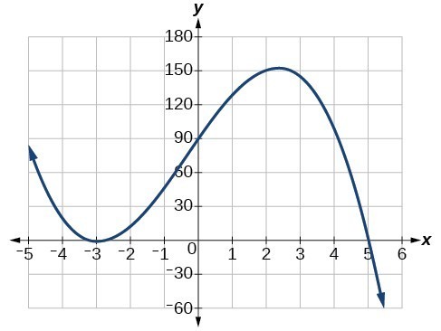
Figure 16
Try It 3
Sketch a graph of [latex]f\left(x\right)=\frac{1}{4}x{\left(x - 1\right)}^{4}{\left(x+3\right)}^{3}[/latex].
Candela Citations
- Precalculus. Authored by: Jay Abramson, et al.. Provided by: OpenStax. Located at: http://cnx.org/contents/fd53eae1-fa23-47c7-bb1b-972349835c3c@5.175. License: CC BY: Attribution. License Terms: Download For Free at : http://cnx.org/contents/fd53eae1-fa23-47c7-bb1b-972349835c3c@5.175.