In some situations, we may know two points on a graph but not the zeros. If those two points are on opposite sides of the x-axis, we can confirm that there is a zero between them. Consider a polynomial function f whose graph is smooth and continuous. The Intermediate Value Theorem states that for two numbers a and b in the domain of f, if a < b and [latex]f\left(a\right)\ne f\left(b\right)[/latex], then the function f takes on every value between [latex]f\left(a\right)[/latex] and [latex]f\left(b\right)[/latex].
We can apply this theorem to a special case that is useful in graphing polynomial functions. If a point on the graph of a continuous function f at [latex]x=a[/latex] lies above the x-axis and another point at [latex]x=b[/latex] lies below the x-axis, there must exist a third point between [latex]x=a[/latex] and [latex]x=b[/latex] where the graph crosses the x-axis. Call this point [latex]\left(c,\text{ }f\left(c\right)\right)[/latex]. This means that we are assured there is a solution c where [latex]f\left(c\right)=0[/latex].
In other words, the Intermediate Value Theorem tells us that when a polynomial function changes from a negative value to a positive value, the function must cross the x-axis. Figure 17 shows that there is a zero between a and b.
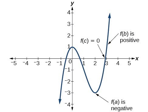
Figure 17. Using the Intermediate Value Theorem to show there exists a zero.
A General Note: Intermediate Value Theorem
Let f be a polynomial function. The Intermediate Value Theorem states that if [latex]f\left(a\right)[/latex] and [latex]f\left(b\right)[/latex] have opposite signs, then there exists at least one value c between a and b for which [latex]f\left(c\right)=0[/latex].
Example 9: Using the Intermediate Value Theorem
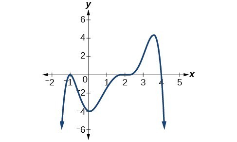
Show that the function [latex]f\left(x\right)={x}^{3}-5{x}^{2}+3x+6[/latex] has at least two real zeros between [latex]x=1[/latex] and [latex]x=4[/latex].
Solution
As a start, evaluate [latex]f\left(x\right)[/latex] at the integer values [latex]x=1,2,3,\text{ and }4[/latex].
| x | 1 | 2 | 3 | 4 |
| f (x) | 5 | 0 | –3 | 2 |
We see that one zero occurs at [latex]x=2[/latex]. Also, since [latex]f\left(3\right)[/latex] is negative and [latex]f\left(4\right)[/latex] is positive, by the Intermediate Value Theorem, there must be at least one real zero between 3 and 4.
We have shown that there are at least two real zeros between [latex]x=1[/latex] and [latex]x=4[/latex].
Try It 4
Show that the function [latex]f\left(x\right)=7{x}^{5}-9{x}^{4}-{x}^{2}[/latex] has at least one real zero between [latex]x=1[/latex] and [latex]x=2[/latex].
Writing Formulas for Polynomial Functions
Now that we know how to find zeros of polynomial functions, we can use them to write formulas based on graphs. Because a polynomial function written in factored form will have an x-intercept where each factor is equal to zero, we can form a function that will pass through a set of x-intercepts by introducing a corresponding set of factors.
A General Note: Factored Form of Polynomials
If a polynomial of lowest degree p has horizontal intercepts at [latex]x={x}_{1},{x}_{2},\dots ,{x}_{n}[/latex], then the polynomial can be written in the factored form: [latex]f\left(x\right)=a{\left(x-{x}_{1}\right)}^{{p}_{1}}{\left(x-{x}_{2}\right)}^{{p}_{2}}\cdots {\left(x-{x}_{n}\right)}^{{p}_{n}}[/latex] where the powers [latex]{p}_{i}[/latex] on each factor can be determined by the behavior of the graph at the corresponding intercept, and the stretch factor a can be determined given a value of the function other than the x-intercept.
How To: Given a graph of a polynomial function, write a formula for the function.
- Identify the x-intercepts of the graph to find the factors of the polynomial.
- Examine the behavior of the graph at the x-intercepts to determine the multiplicity of each factor.
- Find the polynomial of least degree containing all the factors found in the previous step.
- Use any other point on the graph (the y-intercept may be easiest) to determine the stretch factor.
Example 10: Writing a Formula for a Polynomial Function from the Graph
Write a formula for the polynomial function shown in Figure 19.
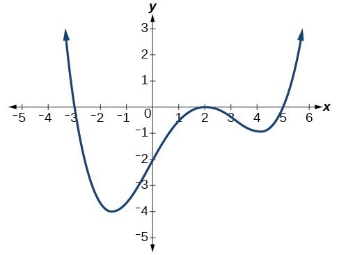
Figure 19
Solution
This graph has three x-intercepts: x = –3, 2, and 5. The y-intercept is located at (0, 2). At x = –3 and x = 5, the graph passes through the axis linearly, suggesting the corresponding factors of the polynomial will be linear. At x = 2, the graph bounces at the intercept, suggesting the corresponding factor of the polynomial will be second degree (quadratic). Together, this gives us
To determine the stretch factor, we utilize another point on the graph. We will use the y-intercept (0, –2), to solve for a.
The graphed polynomial appears to represent the function [latex]f\left(x\right)=\frac{1}{30}\left(x+3\right){\left(x - 2\right)}^{2}\left(x - 5\right)[/latex].
Using Local and Global Extrema
With quadratics, we were able to algebraically find the maximum or minimum value of the function by finding the vertex. For general polynomials, finding these turning points is not possible without more advanced techniques from calculus. Even then, finding where extrema occur can still be algebraically challenging. For now, we will estimate the locations of turning points using technology to generate a graph.
Each turning point represents a local minimum or maximum. Sometimes, a turning point is the highest or lowest point on the entire graph. In these cases, we say that the turning point is a global maximum or a global minimum. These are also referred to as the absolute maximum and absolute minimum values of the function.
Local and Global Extrema
A local maximum or local minimum at x = a (sometimes called the relative maximum or minimum, respectively) is the output at the highest or lowest point on the graph in an open interval around x = a. If a function has a local maximum at a, then [latex]f\left(a\right)\ge f\left(x\right)[/latex] for all x in an open interval around x = a. If a function has a local minimum at a, then [latex]f\left(a\right)\le f\left(x\right)[/latex] for all x in an open interval around x = a.
A global maximum or global minimum is the output at the highest or lowest point of the function. If a function has a global maximum at a, then [latex]f\left(a\right)\ge f\left(x\right)[/latex] for all x. If a function has a global minimum at a, then [latex]f\left(a\right)\le f\left(x\right)[/latex] for all x.
We can see the difference between local and global extrema in Figure 21.
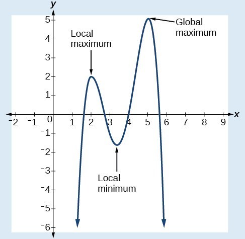
Figure 21
Q & A
Do all polynomial functions have a global minimum or maximum?
No. Only polynomial functions of even degree have a global minimum or maximum. For example, [latex]f\left(x\right)=x[/latex] has neither a global maximum nor a global minimum.
Example 11: Using Local Extrema to Solve Applications
An open-top box is to be constructed by cutting out squares from each corner of a 14 cm by 20 cm sheet of plastic then folding up the sides. Find the size of squares that should be cut out to maximize the volume enclosed by the box.
Solution
We will start this problem by drawing a picture like Figure 22, labeling the width of the cut-out squares with a variable, w.
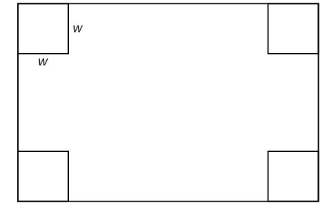
Figure 22
Notice that after a square is cut out from each end, it leaves a [latex]\left(14 - 2w\right)[/latex] cm by [latex]\left(20 - 2w\right)[/latex] cm rectangle for the base of the box, and the box will be w cm tall. This gives the volume
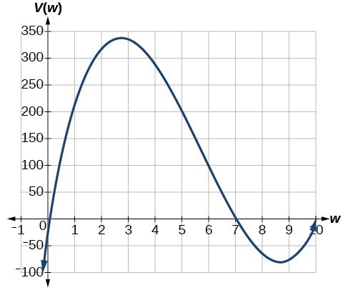
Figure 23
Notice, since the factors are w, [latex]20 - 2w[/latex] and [latex]14 - 2w[/latex], the three zeros are 10, 7, and 0, respectively. Because a height of 0 cm is not reasonable, we consider the only the zeros 10 and 7. The shortest side is 14 and we are cutting off two squares, so values w may take on are greater than zero or less than 7. This means we will restrict the domain of this function to [latex]0
From this graph, we turn our focus to only the portion on the reasonable domain, [latex]\left[0,\text{ }7\right][/latex]. We can estimate the maximum value to be around 340 cubic cm, which occurs when the squares are about 2.75 cm on each side. To improve this estimate, we could use advanced features of our technology, if available, or simply change our window to zoom in on our graph to produce the graph in Figure 24.
![Graph of V(w)=(20-2w)(14-2w)w where the x-axis is labeled w and the y-axis is labeled V(w) on the domain [2.4, 3].](https://s3-us-west-2.amazonaws.com/courses-images-archive-read-only/wp-content/uploads/sites/924/2015/11/25201457/CNX_Precalc_Figure_03_04_0292.jpg)
Figure 24
From this zoomed-in view, we can refine our estimate for the maximum volume to about 339 cubic cm, when the squares measure approximately 2.7 cm on each side.
Try It 6
Use technology to find the maximum and minimum values on the interval [latex]\left[-1,4\right][/latex] of the function [latex]f\left(x\right)=-0.2{\left(x - 2\right)}^{3}{\left(x+1\right)}^{2}\left(x - 4\right)[/latex].
Candela Citations
- Precalculus. Authored by: Jay Abramson, et al.. Provided by: OpenStax. Located at: http://cnx.org/contents/fd53eae1-fa23-47c7-bb1b-972349835c3c@5.175. License: CC BY: Attribution. License Terms: Download For Free at : http://cnx.org/contents/fd53eae1-fa23-47c7-bb1b-972349835c3c@5.175.
Analysis of the Solution
We can also see in Figure 18 that there are two real zeros between [latex]x=1[/latex] and [latex]x=4[/latex].
Figure 18