Graphing the Polar Equations of Conics

When graphing in Cartesian coordinates, each conic section has a unique equation. This is not the case when graphing in polar coordinates. We must use the eccentricity of a conic section to determine which type of curve to graph, and then determine its specific characteristics. The first step is to rewrite the conic in standard form as we have done in the previous example. In other words, we need to rewrite the equation so that the denominator begins with 1. This enables us to determine $e$ and, therefore, the shape of the curve. The next step is to substitute values for $\theta$ and solve for $r$ to plot a few key points. Setting $\theta$ equal to $0,\frac{\pi }{2},\pi$ , and $\frac{3\pi }{2}$ provides the vertices so we can create a rough sketch of the graph.

Example 2: Graphing a Parabola in Polar Form

Graph $r=\frac{5}{3+3\text{ }\cos \text{ }\theta }$ .

Solution

First, we rewrite the conic in standard form by multiplying the numerator and denominator by the reciprocal of 3, which is $\frac{1}{3}$ .

$\begin{array}{l}\begin{array}{l}\hfill \\ \hfill \\ r=\frac{5}{3+3\text{ }\cos \text{ }\theta }=\frac{5\left(\frac{1}{3}\right)}{3\left(\frac{1}{3}\right)+3\left(\frac{1}{3}\right)\cos \text{ }\theta }\hfill \end{array}\hfill \\ r=\frac{\frac{5}{3}}{1+\cos \text{ }\theta }\hfill \end{array}$

Because $e=1$ , we will graph a parabola with a focus at the origin. The function has a $\cos \text{ }\theta$ , and there is an addition sign in the denominator, so the directrix is $x=p$ .

$\begin{array}{l}\frac{5}{3}=ep\\ \frac{5}{3}=\left(1\right)p\\ \frac{5}{3}=p\end{array}$

The directrix is $x=\frac{5}{3}$ .

Plotting a few key points as in the table below will enable us to see the vertices.

	A	B	C	D
$\theta$	$0$	$\frac{\pi }{2}$	$\pi$	$\frac{3\pi }{2}$
$r=\frac{5}{3+3\text{ }\cos \text{ }\theta }$	$\frac{5}{6}\approx 0.83$	$\frac{5}{3}\approx 1.67$	undefined	$\frac{5}{3}\approx 1.67$

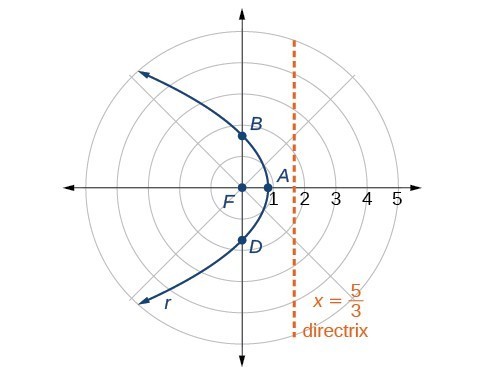
Figure 3

Analysis of the Solution

We can check our result with a graphing utility.

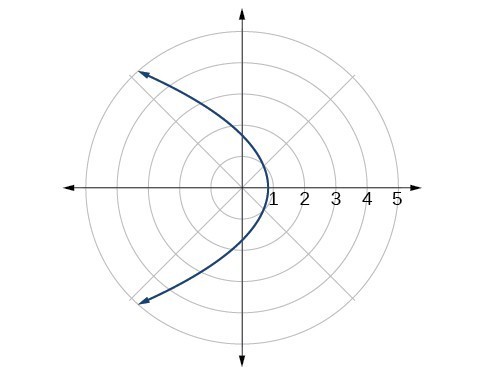
Figure 4

Example 3: Graphing a Hyperbola in Polar Form

Graph $r=\frac{8}{2 - 3\text{ }\sin \text{ }\theta }$ .

Solution

First, we rewrite the conic in standard form by multiplying the numerator and denominator by the reciprocal of 2, which is $\frac{1}{2}$ .

$\begin{array}{l}\begin{array}{l}\hfill \\ \hfill \\ r=\frac{8}{2 - 3\sin \text{ }\theta }=\frac{8\left(\frac{1}{2}\right)}{2\left(\frac{1}{2}\right)-3\left(\frac{1}{2}\right)\sin \text{ }\theta }\hfill \end{array}\hfill \\ r=\frac{4}{1-\frac{3}{2}\text{ }\sin \text{ }\theta }\hfill \end{array}$

Because $e=\frac{3}{2},e>1$ , so we will graph a hyperbola with a focus at the origin. The function has a $\sin \text{ }\theta$ term and there is a subtraction sign in the denominator, so the directrix is $y=-p$ .

$\begin{array}{l}\text{ }4=ep\hfill \\ \text{ }4=\left(\frac{3}{2}\right)p\hfill \\ 4\left(\frac{2}{3}\right)=p\hfill \\ \text{ }\frac{8}{3}=p\hfill \end{array}$

The directrix is $y=-\frac{8}{3}$ .

Plotting a few key points as in the table below will enable us to see the vertices.

	A	B	C	D
$\theta$	$0$	$\frac{\pi }{2}$	$\pi$	$\frac{3\pi }{2}$
$r=\frac{8}{2 - 3\sin \theta }$	$4$	$-8$	$4$	$\frac{8}{5}=1.6$

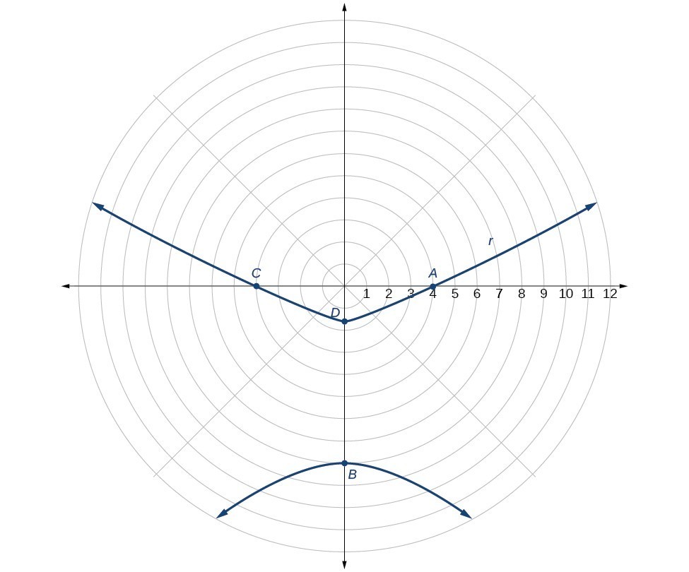
Figure 5

Example 4: Graphing an Ellipse in Polar Form

Graph $r=\frac{10}{5 - 4\text{ }\cos \text{ }\theta }$ .

Solution

First, we rewrite the conic in standard form by multiplying the numerator and denominator by the reciprocal of 5, which is $\frac{1}{5}$ .

$\begin{array}{l}\hfill \\ \begin{array}{l}r=\frac{10}{5 - 4\cos \text{ }\theta }=\frac{10\left(\frac{1}{5}\right)}{5\left(\frac{1}{5}\right)-4\left(\frac{1}{5}\right)\cos \text{ }\theta }\hfill \\ r=\frac{2}{1-\frac{4}{5}\text{ }\cos \text{ }\theta }\hfill \end{array}\hfill \end{array}$

Because $e=\frac{4}{5},e<1$ , so we will graph an ellipse with a focus at the origin. The function has a $\text{cos}\theta$ , and there is a subtraction sign in the denominator, so the directrix is $x=-p$ .

$\begin{array}{l}\text{ }2=ep\hfill \\ \text{ }2=\left(\frac{4}{5}\right)p\hfill \\ 2\left(\frac{5}{4}\right)=p\hfill \\ \text{ }\frac{5}{2}=p\hfill \end{array}$

The directrix is $x=-\frac{5}{2}$ .

Plotting a few key points as in the table below will enable us to see the vertices.

	A	B	C	D
$\theta$	$0$	$\frac{\pi }{2}$	$\pi$	$\frac{3\pi }{2}$
$r=\frac{10}{5 - 4\text{ }\cos \text{ }\theta }$	$10$	$2$	$\frac{10}{9}\approx 1.1$	$2$

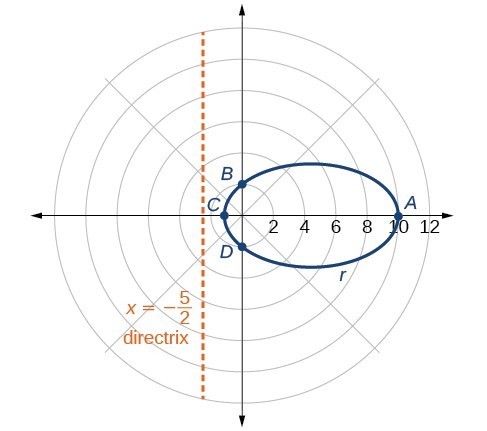
Figure 6

Analysis of the Solution

We can check our result using a graphing utility.

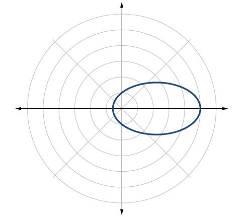
Figure 7. $r=\frac{10}{5 - 4\text{ }\cos \text{ }\theta }$ graphed on a viewing window of $\left[-3,12,1\right]$ by $\left[-4,4,1\right],\theta \text{min =}0$ and $\theta \text{max =}2\pi$ .

Try It 2

Graph $r=\frac{2}{4-\cos \text{ }\theta }$ .

Solution

Conic Sections in Polar Coordinates