As we discussed in the previous page, exponential functions are used for many real-world applications such as finance, forensics, computer science, and most of the life sciences. Working with an equation that describes a real-world situation gives us a method for making predictions. Most of the time, however, the equation itself is not enough. We learn a lot about things by seeing their visual representations, and that is exactly why graphing exponential equations is a powerful tool. It gives us another layer of insight for predicting future events.

Characteristics of Graphs of Exponential Functions

Before we begin graphing, it is helpful to review the behavior of exponential growth. Recall the table of values for a function of the form [latex]f\left(x\right)={b}^{x}[/latex] whose base is greater than one. We’ll use the function [latex]f\left(x\right)={2}^{x}[/latex]. Observe how the output values in the table below change as the input increases by 1.

Each output value is the product of the previous output and the base, 2. We call the base 2 the constant ratio. In fact, for any exponential function with the form [latex]f\left(x\right)=a{b}^{x}[/latex], b is the constant ratio of the function. This means that as the input increases by 1, the output value will be the product of the base and the previous output, regardless of the value of a.

Notice from the table that:

• the output values are positive for all values of x
• as x increases, the output values increase without bound
• as x decreases, the output values grow smaller, approaching zero

The graph below shows the exponential growth function [latex]f\left(x\right)={2}^{x}[/latex].

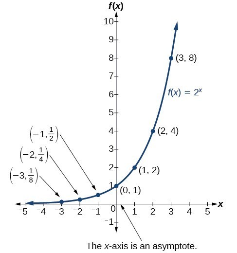
Notice that the graph gets close to the x-axis but never touches it.

The domain of [latex]f\left(x\right)={2}^{x}[/latex] is all real numbers, the range is [latex]\left(0,\infty \right)[/latex], and the horizontal asymptote is [latex]y=0[/latex].

To get a sense of the behavior of exponential decay, we can create a table of values for a function of the form [latex]f\left(x\right)={b}^{x}[/latex] whose base is between zero and one. We’ll use the function [latex]g\left(x\right)={\left(\frac{1}{2}\right)}^{x}[/latex]. Observe how the output values in the table below change as the input increases by 1.

Again, because the input is increasing by 1, each output value is the product of the previous output and the base or constant ratio [latex]\frac{1}{2}[/latex].

Notice from the table that:

• the output values are positive for all values of x
• as x increases, the output values grow smaller, approaching zero
• as x decreases, the output values grow without bound

The graph below shows the exponential decay function, [latex]g\left(x\right)={\left(\frac{1}{2}\right)}^{x}[/latex].

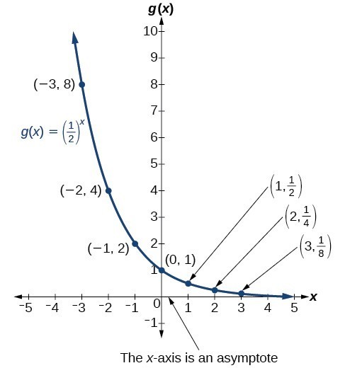
The domain of [latex]g\left(x\right)={\left(\frac{1}{2}\right)}^{x}[/latex] is all real numbers, the range is [latex]\left(0,\infty \right)[/latex], and the horizontal asymptote is [latex]y=0[/latex].

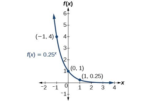
Example: Sketching the Graph of an Exponential Function of the Form [latex]f\left(x\right)={b}^{x}[/latex]

Sketch a graph of [latex]f\left(x\right)={0.25}^{x}[/latex]. State the domain, range, and asymptote.

Show Solution

Before graphing, identify the behavior and create a table of points for the graph.

• Since b = 0.25 is between zero and one, we know the function is decreasing. The left tail of the graph will increase without bound, and the right tail will approach the asymptote y = 0.
• Create a table of points.
  

  x	–3	–2	–1	0	1	2	3
  [latex]f\left(x\right)={0.25}^{x}[/latex]	64	16	4	1	0.25	0.0625	0.015625

• Plot the y-intercept, [latex]\left(0,1\right)[/latex], along with two other points. We can use [latex]\left(-1,4\right)[/latex] and [latex]\left(1,0.25\right)[/latex].

Draw a smooth curve connecting the points.

The domain is [latex]\left(-\infty ,\infty \right)[/latex], the range is [latex]\left(0,\infty \right)[/latex], and the horizontal asymptote is [latex]y=0[/latex].

Try It

Sketch the graph of [latex]f\left(x\right)={4}^{x}[/latex]. State the domain, range, and asymptote.

Show Solution

The domain is [latex]\left(-\infty ,\infty \right)[/latex], the range is [latex]\left(0,\infty \right)[/latex], and the horizontal asymptote is [latex]y=0[/latex].

Bounded Growth

Exponential growth cannot continue forever. Exponential models, while they may be useful in the short term, tend to fall apart the longer they continue. Consider an aspiring writer who writes a single line on day one and plans to double the number of lines she writes each day for a month. By the end of the month, she must write over 17 billion lines or one-half-billion pages. It is impractical, if not impossible, for anyone to write that much in such a short period of time. Eventually, most models like this begin to approach some limiting value and then the growth is forced to slow. For this reason, it is often better to use a model with an upper bound instead of an exponential growth model although the exponential growth model is still useful over a short term before approaching the limiting value.

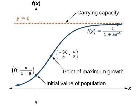
The logistic growth model is approximately exponential at first, but it has a reduced rate of growth as the output approaches the model’s upper bound called the carrying capacity. For constants a, b, and c, the logistic growth of a population over time x is represented by the model

[latex]f\left(x\right)=\frac{c}{1+a{e}^{-bx}}[/latex]

The graph below shows how the growth rate changes over time. The graph increases from left to right, but the growth rate only increases until it reaches its point of maximum growth rate at which the rate of increase decreases.

Example: Using the Logistic-Growth Model

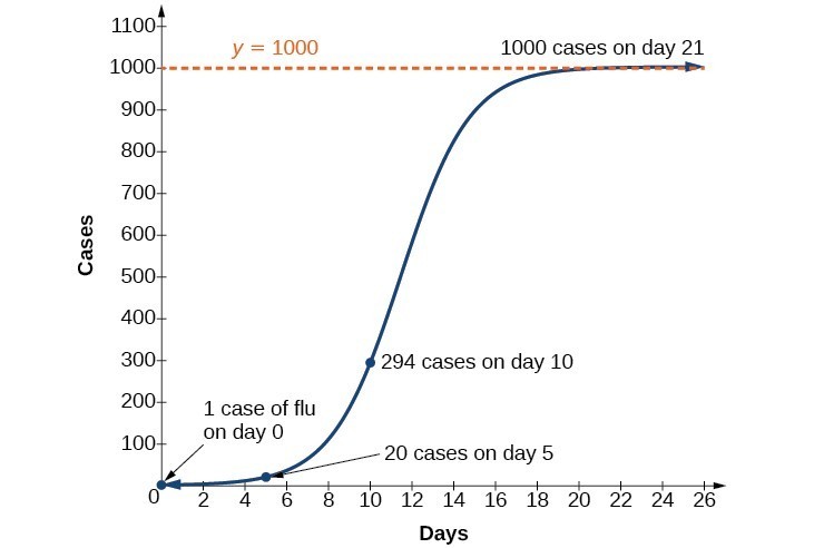
An influenza epidemic spreads through a population rapidly at a rate that depends on two factors. The more people who have the flu, the more rapidly it spreads, and also the more uninfected people there are, the more rapidly it spreads. These two factors make the logistic model good for studying the spread of communicable diseases. And, clearly, there is a maximum value for the number of people infected: the entire population.

For example, at time t = 0 there is one person in a community of 1,000 people who has the flu. So, in that community, at most 1,000 people can have the flu. Researchers find that for this particular strain of the flu, the logistic growth constant is b = 0.6030. Estimate the number of people in this community who will have had this flu after ten days. Predict how many people in this community will have had this flu after a long period of time has passed.

Show Solution

We substitute the given data into the logistic growth model

[latex]f\left(x\right)=\frac{c}{1+a{e}^{-bx}}[/latex]

Because at most 1,000 people, the entire population of the community, can get the flu, we know the limiting value is c = 1000. To find a, we use the formula that the number of cases at time t = 0 is [latex]\frac{c}{1+a}=1[/latex], from which it follows that a = 999. This model predicts that, after ten days, the number of people who have had the flu is [latex]f\left(x\right)=\frac{1000}{1+999{e}^{-0.6030x}}\approx 293.8[/latex]. Because the actual number must be a whole number (a person has either had the flu or not) we round to 294. In the long term, the number of people who will contract the flu is the limiting value, c = 1000.

Analysis of the Solution

Remember that because we are dealing with a virus, we cannot predict with certainty the number of people infected. The model only approximates the number of people infected and will not give us exact or actual values.

The graph below gives a good picture of how this model fits the data.

The graph of [latex]f\left(x\right)=\frac{1000}{1+999{e}^{-0.6030x}}[/latex].

Key Equations

Key Concepts

• • • An exponential function is defined as a function with a positive constant other than 1 raised to a variable exponent.
    • Scientific and graphing calculators have the key [latex]\left[{e}^{x}\right][/latex] or [latex]\left[\mathrm{exp}\left(x\right)\right][/latex] for calculating powers of e.
    • Continuous growth or decay models are exponential models that use e as the base. Continuous growth and decay models can be found when the initial value and growth or decay rate are known.
    • The graph of the function [latex]f\left(x\right)={b}^{x}[/latex] has a y-intercept at [latex]\left(0, 1\right)[/latex], domain of [latex]\left(-\infty , \infty \right)[/latex], range of [latex]\left(0, \infty \right)[/latex], and horizontal asymptote of [latex]y=0[/latex].
    • If [latex]b>1[/latex], the function is increasing. The left tail of the graph will approach the asymptote [latex]y=0[/latex], and the right tail will increase without bound.
    • If 0 < b < 1, the function is decreasing. The left tail of the graph will increase without bound, and the right tail will approach the asymptote [latex]y=0[/latex].
    • We can use logistic growth functions to model real-world situations where the rate of growth changes over time, such as population growth, spread of disease, and spread of rumors.

Glossary

carrying capacity

in a logistic model, the limiting value of the output

logistic growth model

a function of the form [latex]f\left(x\right)=\frac{c}{1+a{e}^{-bx}}[/latex] where [latex]\frac{c}{1+a}[/latex] is the initial value, c is the carrying capacity, or limiting value, and b is a constant determined by the rate of growth