Learning Outcomes
- Use a spreadsheet to create a scatterplot
- Use a spreadsheet to generate a trendline for a scatterplot
- Analyze a trendline for appropriateness and fit
ordered pairs as coordinates for data points in the plane
Recall that ordered pairs in the form [latex]\left(x, y\right)[/latex] give information about a point in the plane.
The graph of an equation contains a set of such points having input, [latex]x[/latex]-values and corresponding output, [latex]y[/latex]-values. Each ordered pair (data point) on the graph of such a mathematical relation satisfies the equation of the relation (makes it a true statement when substituted for the variables).
In many real-world situations a dependent relationship can be identified between two quantities, the independent variable and the dependent variable.

Image credit: Christopher Ziemnowicz
For example, say you purchase a brand-new car from a dealership. The value of your car begins to decline as soon as you sign the sales contract and drive the car off the lot. Notwithstanding other variables such as vehicle damage or economic fluctuations, the value of your new car going forward will be largely dependent upon how long you’ve owned it. This type of decrease in value over time is called depreciation.
Populations are also dependent upon time. It is not difficult to visualize growth in the population of people on the Earth over decades and centuries or of a number of bacteria in a petri dish over minutes and hours. Other types of growth depend on quantities other than time. For example, revenue, the amount of money collected when you sell an item, depends upon the number of items sold. The growth (or decay, as in the value of your new car over time) in each of these situations can be modeled mathematically.


In each of these situations the independent variable, representing the input quantity (time in years or number of pizzas sold) is graphed on the horizontal axis while the dependent variable, representing the output quantity (percent of new car value, population, or revenue) is graphed on the vertical axis. Each point on the graph represents a correspondence between one piece of information from the set of input values with one piece of information from the set of output values. This correspondence, called a relation, is written in the form of an ordered pair as (input, output) and it satisfies the mathematical statement of the relation between the two quantities described by the equation. A well-defined relation with no ambiguity regarding the output variable is also called a function.
function notation
The notation [latex]y=f\left(x\right)[/latex] defines a function named [latex]f[/latex]. This is read as “[latex]y[/latex] is a function of [latex]x[/latex].” The letter [latex]x[/latex] represents the input value, or independent variable. The letter [latex]y[/latex] or [latex]f\left(x\right)[/latex], represents the output value, or dependent variable.
There are several terms used to denote the coordinates of an ordered pair, (input, output), depending on the discipline applying the math or the particular situation to which it is being applied. You may see them variously referred to as any of the following:
[latex]\left(x, y\right) \quad \left(x, f\left(x\right)\right) \quad \left(t, p\left(t\right)\right) \quad\left(\text{input,} \text{ output}\right) \quad \left(\text{explanatory variable,}\text{ response variable}\right) \quad[/latex].
The letters or terms for the coordinates may change depending on the situation, but conceptually they all represent ordered pairs containing a coordinate from the set of all inputs to the relation along with its corresponding coordinate from the set of all outputs of the relation. A relation in which there is a correspondence between two variables is sometimes called bivariate.
We don’t know what the equation is when we begin to build a model. Instead, we use what we know of the nature of the situation to choose a type of equation or function to apply, and what we observe in the data of the situation to write a particular equation that best fits it. Some situations will be best approximated by linear relationships, that is by equations of lines, while others will require a non-linear relationship such as an exponential function. You will become familiar with linear, exponential, and logistic modeling in this section but you should know that these three types of relationships are just a few of the many types of equations that can be used to model real-world situations.
Let’s begin to get familiar with the tools of modeling while spending some time with the vocabulary and processes of modeling.
Scatterplots
A scatterplot is a graph of plotted points obtained from the real-world situation of interest. Recall an example from the linear (algebraic) growth section of the previous module in which data had been collected on gasoline consumption in the US between the years 1992 and 2004.
| Year | ’92 | ’93 | ’94 | ’95 | ’96 | ’97 | ’98 | ’99 | ’00 | ’01 | ’02 | ’03 | ’04 |
| Consumption (billion of gallons) | 110 | 111 | 113 | 116 | 118 | 119 | 123 | 125 | 126 | 128 | 131 | 133 | 136 |
In the solution to that example, you were shown a graph plotted with data points in the form (year, consumption). Then you were asked to write the recursive and explicit forms to find a model for the data and use it to answer a question. It is important to understand how such a model can be built by hand. As the situations into which we seek insight become more complicated, though, technology can be of tremendous assistance. This module will help you apply your understanding of the characteristics of models by using a spreadsheet to handle the task of developing models fairly quickly and neatly. The examples in this module will use the Microsoft Excel spreadsheet but you can also use an open source spreadsheet such as Apache OpenOffice Calc or Google Sheets. We’ll walk through the basics using the gasoline consumption example.
Spreadsheet Hands-On: Create a Scatterplot
Step 1: Storing the data.
Open a new blank worksheet and save it somewhere safe. You should save your work frequently as you go or turn on an auto-save feature if available. We’ll begin by typing the data from the gasoline consumption example into two columns, one labeled year and the other labeled consumption.
- In cell B1 of your spreadsheet, type the word “Year.” In cell C2, type “Consumption.” Leave column A blank for now.
- Beginning in cell B2, type the consecutive years from 1992 to 2004 each into a cell of its own, straight down. Spreadsheets have a feature to accomplish this quickly. Type just the first two cells, 1992 and 1993. Then highlight both. Grab the little “handle” in the lower right corner of the outline of the highlighted cells and drag it down to populate the remaining cells by continuing the series. In fact, in Excel, if you click the box that appears after populating a few cells, you get options for how you’d like for them to be filled: each a copy of the other, or a series as we just did.


- Beginning in cell C2, type the consumption quantity that corresponds to each year.When you are done it should look like the image below. Click on any image on the page for a closer view in a new tab.


Step 2: Creating the scatterplot.
Click and drag to highlight cells B1 and C1 containing the words “year” and “consumption” then drag downward to highlight all the data points you entered.
- Click “Insert” on the task ribbon then choose Scatter under the Charts block, and click the first scatter icon, Scatter.
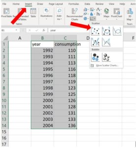
- A plot should appear showing each of your data points above their corresponding years.
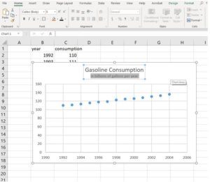
- You can change the formatting of the chart now or later. Let’s take care of the title while we have it open in front of us. Click on the word “consumption: and change the title of the chart by typing over the existing title. Let’s change it to “Gasoline Consumption in billions of gallons per year.” See the image below. You can obtain the subtitle text by shift-entering after the word “Consumption” then change it to a smaller font by selecting just the text you want to make small and changing its font size in the Home tab on the ribbon.
- You can play around with the settings to adjust the color scheme and style of the chart elements by clicking on the chart and choosing the style box with a paintbrush icon that appears to the right of the chart or by clicking on the Design and Format tabs in the ribbon

You’ve just created a scatterplot of known data points in the gas consumption scenario. This scatterplot will make a nice presentation in a report or a display, but we’ll need to make an adjustment to the input data to be able to obtain an meaningful equation to use as a model. We’ll see how to choose an equation type to use to model the situation next.
Trendlines
Trendlines in a spreadsheet chart represent graphs that nicely fit the data of your scatterplot, like the line of best fit you discovered when you completed this gasoline consumption scenario in the previous module. In that example, you visually inspected the scatterplot for a pattern and noticed that the data very nearly approximated a straight line. You chose two data points and used them to write the recursive and explicit forms of the linear relationship present in the data. Starting with 111 billion gallons consumed in the year 1993, you found the slope to be [latex]2.2[/latex] billion gallons of gas consumed per year: [latex]P_{n}=111+2.2n[/latex].
Function notation and subscripts
In the equation above, [latex]P_{n}=111+2.2n[/latex], the output variable is represented as [latex]P[/latex] per unit of input [latex]n[/latex]. We could have just as appropriately written it as [latex]P\left(n\right)=111+2.2n[/latex] or even as [latex]y=111+2.2n[/latex].
We need to adjust the data that our chart is using for the input values. We currently have a list of years in the input column, which yields a nice presentation of the data but, If we wish to obtain an equation to use as a model for this situation, we need to change the perspective of our input to get a more meaningful mathematical statement. We’ll need to change the input information from years to the number of years after a starting year.
Let’s see what equation we obtain when we let Excel choose the line that best fits the data. In this example, we will obtain an unexpected result in step 1, then we’ll adjust the chart to fix it in step 2.
Spreadsheet Hands-On: Choose a trendline
Step 1: Selecting the trendline from a menu.
Click on the chart you made previously then click on the topmost style box that appears, the one with a plus-sign in it, to open the Chart Elements box. Hover your mouse over the Trendline choice, click the right-arrow, then choose More Options… to open the Format Trendline pane.

- Click the radio button next to the Linear trendline option.
- Click “Display Equation on chart.”
- Click “Display R-Squared value on chart.”
When you’ve made those choices it should look like the image below. You can close the Format Trendline pane at this point. Excel places the equation and R-Squared value directly over the scatterplot, making it difficult to read. You can click the textbox containing them and move it down if you wish.

Excel has given us a trendline equation of [latex]y=2.1758x-4225.1[/latex] and an R-Squared value of [latex]0.9946[/latex]. The R-Squared value is a measure of how well the trendline fits the data: the closer to [latex]1[/latex], the better. an R-Squared value of [latex]0.9946[/latex] indicates that our data very closely matches the trendline. But what about the equation? It differs from the explicit form you wrote when you completed this example previously. We’ll examine why, then make an adjustment to the chart so that they match more closely.
Step 2: Analyzing the trendline
The trendline that Excel gave us is [latex]y=2.1758x-4225.1[/latex]. This equation follows the form of a linear equation, [latex]y=mx+b[/latex], with slope of [latex]2.1758[/latex] and an initial value of [latex]-4225.1[/latex]. The slope is similar to the slope of [latex]2.2[/latex] we obtained by hand in the previous module, but the constant is way off, and negative. Why is that?
Excel is reading the input values as numbers, not as we are perceiving them, as years. That is, the software interprets the number 1993 as one thousand nine-hundred ninety-three years after the starting year, year zero. We want it to read 1993 as the first input so that we have a starting value of approximately 111. We’ll need to change our data from years to years since 1993 to match the equation we obtained earlier. Recall that you left column A empty in the beginning. Let’s use it now.
Step 3: Adjusting the data source
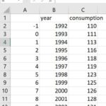
- Since we want to make the gas consumption in the year 1993 our starting value for the equation, we need to start with the data point [latex](0, 111)[/latex]. This will mean the quantity consumed in 1992 will correspond to an input of [latex]-1[/latex], one year prior to 1993. Type [latex]-1[/latex] in cell A2 and [latex]0[/latex] in cell A3, then grab the handle and fill the series down to cell A14. It should look like the image below.
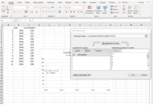
- Right-click on your chart and choose Select Data from the menu that appears.
- Click the word Edit in the Legend Entries (Series) tab ribbon to open the Edit Series box.
- Note that the Series X values row (the middle row shown) is currently populated with values in Sheet6!$B$2:$B$14. (Your sheet number will be different, and will correspond to the name of the sheet tab at the bottom of your page. For example, if you had renamed Sheet1 to Gas, your X values series data would be listed as =Gas!$B$2:$B$14.) The idea is that the spreadsheet is populating the input axis with the numbers found in column B, as shown in the image below.
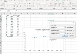
We need for it to instead use the numbers in column A. You can edit the row by changing the two Bs to As. Click OK. The Select Data Source box reappears and you can see that the data for the Horizontal (Category) Axis Labels now includes the data in column A (see below).
- Click OK in the Select Data Source Box. As you do so, note that the highlight box that had been on column B has moved to column A, indicating that’s where the data is now sourced. But the graph is blank. We need to adjust the input starting value, which is still starting from [latex]1990[/latex].
- Click on your chart then double-click on any number in the horizontal axis label text box to open the Format Axis pane. Under Axis Options, Bounds, click the Reset button to set the minimum to [latex]-1[/latex] and the Maximum to [latex]12[/latex]. The graph should have reappeared as shown below.
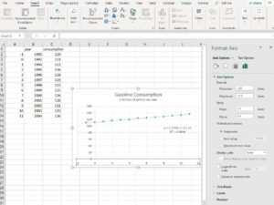 Note the equation of the line of best fit is now [latex]y=2.1758x+111.35[/latex]. This compares very closely to the equation you wrote by hand in the previous module. Let’s examine them.Original explicit form: [latex]P_{n}=111+2.2n[/latex]Excel trendline equation: [latex]y=2.1758x+111.35[/latex].Let [latex]y=P_{n}[/latex] and [latex]x=n[/latex], then we have [latex]P_{n}=111.35+2.1758n[/latex], which is very similar to the equation you wrote by hand.


As you become more familiar working in a spreadsheet, you’ll find using technology to analyze situations numerically is generally more efficient than doing it by hand. But the technology can only act as a tool for your understanding. Without your knowledge of the process of modeling and why it works, the tool is likely to reveal unexpected and confusing results.
Candela Citations
- Authored by: Deborah Devlin. License: CC BY: Attribution
- Screenshot of Excel worksheet. Authored by: Deborah Devlin. License: CC BY: Attribution
- Car dealership in Rockville maryland Jeep.jpg. Authored by: Christopher Ziemnowicz. Located at: https://commons.wikimedia.org/w/index.php?curid=2063231. License: Public Domain: No Known Copyright