Learning Outcomes
- Write a linear model given information about a real-world situation
- Perform linear regression on a data set
- Identify and apply the coefficient of determination
- Identify and apply the correlation coefficient
As you saw in the previous module, situations involving growth (or decay) in which the output quantity changes by a constant amount per unit of input are said to exhibit linear growth. That is, from one input to the next, there is a common difference between the output values.

A Morgan silver dollar
For example, let’s say you inherit a collection of [latex]47[/latex] silver dollars minted between 1878 and 1935. After doing some research, you learn that they are worth between $14 and $30 each. Rather than just cashing them in, you decide to grow the collection by purchasing an additional silver dollar each month. You can write a mathematical model to quickly predict how many silver dollars you’ll have in the collection at any time in the future assuming you increase your collection by [latex]12[/latex] dollars per year. We can write a mathematical model to describe this situation from the information given about the starting amount and the constant quantity of change.
Let the input variable (the independent variable) [latex]x[/latex] represent the number of years you’ve owned the collection of silver dollars. The output variable (the dependent variable) [latex]y[/latex] will represent the total number of dollars in the collection in any year [latex]x[/latex].
| The number of dollars in the collection | is obtained from | the starting number, 47 | together with | 12 more for each year you’ve owned it |
| [latex]y[/latex] | [latex]=[/latex] | [latex]47[/latex] | [latex]+[/latex] | [latex]12\ast x[/latex] |
[latex]y=47+12x[/latex]
Equivalently, in the slope-intercept form of a linear equation,
[latex]y=mx+b[/latex]
[latex]y=12x+47[/latex]
equations of lines in slope-intercept form
- [latex]\displaystyle \text{Slope }=\frac{\text{rise}}{\text{run}}[/latex] and [latex]\displaystyle m=\frac{{{y}_{2}}-{{y}_{1}}}{{{x}_{2}}-{{x}_{1}}}[/latex] where [latex]m=\text{slope}[/latex] and [latex]\displaystyle ({{x}_{1}},{{y}_{1}})[/latex] and [latex]\displaystyle ({{x}_{2}},{{y}_{2}})[/latex] are two points on the line.
- The slope-intercept form of the equation of line is [latex]y=mx+b[/latex] where [latex]m[/latex] represents the slope of the line, [latex]b[/latex] represents the [latex]y[/latex]-intercept, and [latex]x[/latex] and [latex]y[/latex] may be substituted by the coordinates of any point contained on the graph of the equation to satisfy it.
Example
A car is taken to a mechanic for repair. The mechanic charges 140 dollars for parts, plus 33 dollars per hour for labor. Write a linear equation, in slope-intercept form, that models this situation.
Let’s use the model of our silver dollar collection to learn how a spreadsheet can help make predictions quickly and efficiently with a model we have already defined.
Spreadsheet Hands-On: Build a model to make predictions
Step 1: Storing formulas in cells
Open your spreadsheet and click the plus-sign in a circle at the bottom of the window to get a new sheet. You can double-click on the name of the sheet to rename it if you wish.
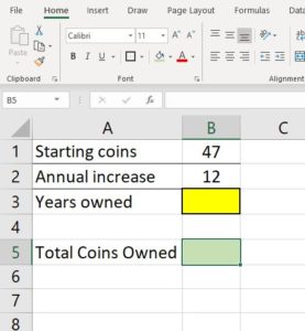
- In cell A1, type “Starting coins.”
- In cell A2, type “Annual increase.”
- In cell A3, type “Years owned.”
- You can play around with various styles of decoration in the Home tab. The width of a column can be increased to the width of the longest cell contents by double-clicking the gray box at the top of the column. Try that on column A. You can also hover your mouse over the edge of the gray area until you get a side-to-side arrow that you can click into an pull the width of the column out or push it in. Here is an example of what it could look like at this stage.
- We will input the formula into cell B5. Formulas in Excel start with an equal symbol “=” that tells the spreadsheet to make a calculation. For example, if you type =5*7 in cell A7 and Enter, the cell will display the result of the multiplication, 35. But if you just type 5*7 without the equal symbol, it will just display 5*7. Try it out now to see how it looks. The “=” tells Excel to do a calculation or perform a formula shortcut. When you are done, delete the contents of A7. We’ll need to use the cell in a little while.
- In cell B5, type =B$2*B$3+B$1 and Enter. The green box should have populated with the number [latex]47[/latex] because we’ve asked it to multiply the value in cell B2 by the value in cell B3 then add the amount in cell B1. And right now, the value in cell B3 should be zero since that cell is empty.
- Now you can use your formula to predict the number of coins owned any number of years after inheriting your collection, assuming you add 12 coins per year to it. How many coins will you have 5 years after inheriting the collection? To answer this question, type the number 5 into cell B3 and Enter. You will have 107 coins 5 years later if you continue diligently to add 12 coins per year.
- You can also use this formula to predict different values. What if you sell 20 of them right away then increase by 12 per year? Or perhaps you keep all 47 but increase by 5 per year instead. The formula will adjust to the new parameters you enter, but it will always return linear growth.

Step 2: Predicting input for a particular output
properties of equality
Recall the properties of equality.
- The addition property of equality states, for all real numbers [latex]a, b, \text{ and } c: \text{ if } a=b \text{, then } a+c=b+c[/latex]. That is, we may add or subtract the same amount to both entire sides of an equation without changing its value.
- The multiplication property of equality states, for all real numbers [latex]a, b, \text{ and } c: \text{ if } a=b \text{, then } a \cdot c=b \cdot c[/latex]. That is, we may multiply or divide the same amount to both entire sides of an equation without changing its value.
- Let’s write a new formula that returns the number of years it will take to reach a certain goal for the total number of coins in the collection.
- In cell A7 (delete any information you put there earlier), type “Coin goal.”
- In cell A8, type “Years required.”
- In our formula [latex]y=12x+47[/latex], we will let [latex]y[/latex] represent the Coin total we desire and solve for [latex]x[/latex].
[latex]\begin{array}{rcl} y&=&12x+47 & \\ y-47&=&12x & \text{subtract 47 on both sides} \\ \dfrac{\left(y-47\right)}{12}&=&x & \text{divide by 12 on both sides} \\ \end{array}[/latex] - Using the formula solved for input, [latex]x=\dfrac{\left(y-47\right)}{12}[/latex], populate cell B8, with the appropriate substitutions for initial value (B1), slope (B2), and desired output (B7). Into cell B8 type, =(B$7-B$1)/B$2 and Enter.
- Set the Coin goal to 500 in cell B7, then Enter. Years required should be 37.75. Then, try adjusting the starting coins and annual increase to see how many or how few years you could reach your goal of 500 total coins.Storing a formula in a spreadsheet is useful for trying out different scenarios and making quick predictions. If the formula is one you use often, a spreadsheet can save you time and energy in the calculations.
Linear Regression
Sometimes writing a formula to represent a particular situation is not an easy task. The situation may be complicated or you just may not have enough information to make the determination that a linear relationship is appropriate for the data. In this case, it is helpful to store the data in a spreadsheet and create a scatterplot as you did in the previous section then let the computer find the appropriate model.
Linear regression is the process of finding the equation of the line that best “fits” the data. Linear regression can be performed simply by “eyeballing” a line that minimizes the distance between the output and the line. We can also use software or a graphing calculator to find this equation. Technology uses a method called Least Squares Regression. This term is not entirely interchangeable the term linear regression but is often used to mean the same thing: finding the line of best fit.
The Correlation Coefficient, [latex]r[/latex], is a value between [latex]-1[/latex] and [latex]1[/latex] that is returned by the least squares method and measures the correlation between the input and output variables of a model. In our linear models, a positive correlation coefficient, [latex]r \gt 0[/latex], would indicate a positive slope while a negative correlation coefficient [latex]r \lt 0[/latex], would indicate a negative slope. Another measure,the square of correlation coefficient [latex]r^2[/latex], is called the Coefficient of Determination. This value is an indicator of how appropriate the regression line is as a model for the situation presented by the data. It ranges from 0 (not at all appropriate) to 1 (perfectly appropriate) as a measure of the proportion of output variability that can be explained by the input in the model. The coefficient of determination is often expressed as a percentage.
Let’s look at an example of using a spreadsheet to perform linear regression on a data set.
The following set of data represents the annual sales of a company in millions of dollars since the year 2003. Let [latex]y[/latex] represent the quantity of sales and let [latex]x[/latex] represent the number of years since 2003.
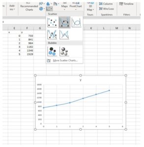
| [latex]x[/latex] | 0 | 1 | 2 | 3 | 4 | 5 |
| [latex]y[/latex] | 733 | 841 | 964 | 1162 | 1346 | 1529 |
Using the techniques you learned in the previous section, store the data in a spreadsheet and use the computer to find the regression line (also called a trendline).
Spreadsheet Hands-On: Use Excel to find the regression line
Step 1: Store the data
- As you did before, label two columns with the the input and the output of the data table. Then highlight both columns at once and choose Scatter with Smooth Lines.
- Click on the chart, then on the style icon with the plus-sign on it, hover over Trendline, click the right arrow, and choose More Options… to open the Format Trendline pane.
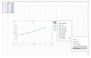
- Choose Linear under Trendline Options, then click Display Equation on chart and Display R-squared value on chart.
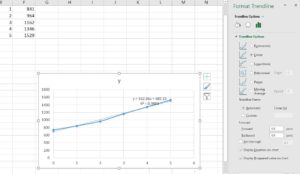
- Note that the equation of the regression line is [latex]y = 162.66x+689.19[/latex] and the [latex]r^2[/latex] value is [latex]0.9881[/latex] (Excel uses a capital R for the coefficient of determination, but we will use a lower-case [latex]r[/latex]). What does the coefficient of determination [latex]r^2[/latex] tell us about the appropriateness of the regression line to model the data? Since [latex]0.9881[/latex] is very close to [latex]1[/latex], this model is a good fit for the data. A coefficient of determination greater than [latex]0.7[/latex] is usually considered good, but there are cases in which a large [latex]r^2[/latex] doesn’t explain well and when a small [latex]r^2[/latex] is considered sufficient. Each situation is different.


In this case, we can use the model to make predictions about the situation. It should be used with caution though, as the only factual information we possess is the data collected. When we make predictions outside a data set, we are said to be extrapolating from the data, which is irresponsible to rely upon as though the prediction is factual. Making predictions within the known data, called interpolating, is much safer since models tend to experience model breakdown, an input beyond which the predicted output does not make sense.
We can also use graphing calculators to perform linear regression. The following video provides an example.
TRY IT
Candela Citations
- Authored by: Deborah Devlin. License: CC BY: Attribution
- Screenshot of Excel Worksheet. Authored by: Deborah Devlin. License: CC BY: Attribution
- Creating a Scatterplot and Performing Liner Regressions. Authored by: James Sousa (Mathispower4u.com). Located at: https://youtu.be/l1QuwXgnSzs. License: CC BY: Attribution
- Morgan silver dollar.jpg. Located at: https://commons.wikimedia.org/w/index.php?curid=965353. License: Public Domain: No Known Copyright
- Question ID 19239. Authored by: Sousa, James. License: CC BY: Attribution. License Terms: IMathAS Community License CC-BY + GPL