While linear regression is a commonly and widely used tool in modeling and data analysis, some data sets are better modeled by non-linear equations. There are several non-linear equations that can be used to model growth. We’ll take a look in this section at one of them: exponential growth.

Imagine growth in a population of bacteria. This kind of single cell life propagates via binary fission. One becomes two, two become four, four become eight, and so on. The population expands rapidly. This is an example of exponential growth. That is, a quantity that grows (or decays) in proportion to itself per unit of input.

We see exponential growth (and decay) in the real world in other situations as well. It shows up in short-run population growth among people and animals, interest earned in banking, radioactive decay, and even in the temperature of a cake cooling from the oven. Anything that grows or decays at a rate proportional to itself experiences exponential growth or decay.

Source: NASA Earth Observatory

As an example, consider the population of the United States. According to the U.S. Census Bureau.There were 242.3 million people in the country in 1987. By the year 2019 there were 329.9 million.  At what rate was the population growing? A few more data points would be helpful to get a good model. A little research at the Census Bureau website revealed the following population counts, [latex]y[/latex], for years [latex]x[/latex] since 1987.

Let’s plot this data on a scatterplot in Excel and perform an exponential regression.

Exponential regression is the process of fitting an exponential function to a set of data. It is performed using the software in a spreadsheet or graphing calculator.

Spreadsheet Hands-On: Perform exponential regression on a population growth

Step 1: Store the data in Excel and create a scatterplot and trendline

1. Open a new spreadsheet or Excel workbook and make two columns for the population data listed above in columns B and C (leave column A blank for now). You can title column B “yrs after 1987” and column C “population in millions.” Store the data underneath each column heading.
2. In column A, type the formula ” =1987+B2″ and Enter. Grab the fill handle in the lower right corner of the cell and pull it down to cell A12. This will fill in the actual years that correspond to each input value. Doing this won’t affect the model, but it will make it easier to interpret visually.
3. Highlight the data, choose the Insert tab in the ribbon at the top of the window then choose a scatter plot to get the chart.
4. Click on the chart, then click the style icon with the plus sign. Mouse-over Trendline and click the right-arrow that appears there. Choose More Options… to open the Format Trendline pane.
5. Click the radio button next to Exponential, and click to Display Equation on chart and Display R-squared value on chart.
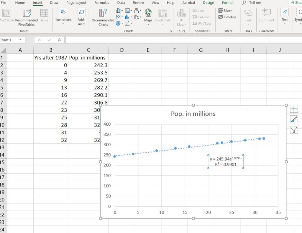
6. The exponential function [latex]y=245.94e^{0.0096x}[/latex] appears with a coefficient of determination [latex]r^{2}=0.9901[/latex]. See below for a discussion of the form of this equation.

Step 2: Convert between continuous and exponential growth

The exponential regression obtained in step six above included a base of [latex]e[/latex]. This base is an irrational number that appears commonly in nature and in exponential growth and decay. It’s approximately equivalent to [latex]2.718[/latex]. But you learned in the previous module that the explicit form of the exponential growth formula is [latex]P_{n}=P_{0}(1+r)^{n}[/latex]. Now we are presented with [latex]y=ae^{x}[/latex], which is called continuous growth. How do these two formulas compare? Let’s look at them side by side.

[latex]P_{n}=P_{0}(1+r)^{n} \qquad \text{ vs. } \qquad y = ae^{rx}[/latex]

We’ll need a fact about exponents before we can discuss them, though.

There are several properties of exponents that allow us to rewrite them in useful ways. Recall that an exponent is a power above a number called a base in the form [latex]a^{m}[/latex]. This tells us to multiply [latex]a[/latex] by itself [latex]m[/latex] times. But, what happens if we raise a base to a power to another power? What does it mean to write [latex]\left(a^{m}\right)^{n}[/latex]?

Consider [latex]\left(a^{3}\right)^{4}[/latex]. Certainly this notation indicates that we should multiply  [latex]\left(a^{3}\right)[/latex] by itself [latex]4[/latex] times.

[latex]\left(a^{3}\right) \ast \left(a^{3}\right) \ast \left(a^{3}\right) \ast \left(a^{3}\right)[/latex]

That yields [latex]\qquad a \cdot a \cdot a \ast a \cdot a \cdot a \ast a \cdot a \cdot a \ast a \cdot a \cdot a = a^{12}[/latex]

So it seems that [latex]\left(a^{3}\right)^{4}=a^{3 \cdot 4}=a^{12}[/latex].

This is a fact. [latex]\left(a^{m}\right)^{n} = a^{m \cdot n}[/latex].

We can leverage this fact to rewrite the form of the exponential equation we obtained above.

[latex]P_{n}=P_{0}(1+r)^{n} \qquad \text{ vs. } \qquad y = ae^{rx}[/latex]

Let [latex]P_{n} = y \text{ and } P_{0} = a \text{ and } n = x[/latex]. Then we have

[latex]y=a(1+r)^{x} \qquad \text{ vs. } \qquad y=ae^{rx}[/latex]

But by the fact that enables us to rewrite exponents, we have that [latex]e^{rx} = \left(e^{r}\right)^{x}[/latex]. This yields

[latex]y=a(1+r)^{x} \qquad \text{ vs. } \qquad y=a\left(e^{r}\right)^{x}[/latex].

Equating the bases in the equations, we can see that certainly, given the same models,

[latex]\left(1+r\right)=e^{r}[/latex].

In the above example regarding the population of the U.S., we should be able to rewrite

[latex]y=245.94e^{0.0096x} \qquad \text{ is equivalent to } \qquad 245.94\left(1.0096\right)^{x}[/latex].

In both the explicit form of exponential growth and the continuous form, we see that the growth rate [latex]r=0.0096[/latex], but this is a coincidence. The two rates will not always be the same number. Furthermore, these are not the same formulas, but they are close enough to one another to be able to approximate in the short run.

Let’s return to the U.S. population from our hands-on spreadsheet example above.

We see that the value of [latex]r^{2}[/latex] is very close to 1, which makes this an appropriate model for the data set, with a starting population of 245.94 million in 1987 and a growth rate of 0.96% per year. But is it a good model for the population growth in the U.S. in general? How confident may we be using this model to extrapolate from the data into the future? Remember that extrapolation can be a risky behavior. According to the Census Bureau, the U.S. grew only 0.62% from Jan. 1, 2018 until Jan. 1, 2019. But the country experienced annual growth rates over 1% during the 1980s. Certainly, growth rates fluctuate over time. Models only approximate growth in the world; they cannot make factual predictions, but they can help us gain insight.

Step 3: Compare exponential regression to linear regression for the same population

1. Click on the chart you built in step 1 above to open the Format Trendline Pane again. This time, choose Linear instead of Exponential. Display the equation and R-squared value.
2. Which trendline offered the higher R-squared value?
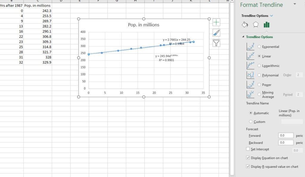
   The linear model [latex]y=2.7661x+244.25[/latex] has an [latex]r^{2}[/latex] of [latex]0.9964[/latex], which is higher than the [latex]r^{2}[/latex] for the exponential regression. Does this make the linear trendline a better model for the population growth? In the short-run, for this particular data set, the lineal model is a better fit. Let’s extrapolate our data into the future and see how many people each model predicts will inhabit the U.S. in the year 2045.

Step 3: Use a model to make a prediction

The calculations we need to make predictions can be done in a spreadsheet or on a calculator. Follow the steps below to see how to use Excel to predict the population in the year 2045, which is 58 years after 1987. We need to substitute 58 for x in each model and see what it predicts.

1. Choose any blank cell to use as a calculator.
2. To calculate the linear model, type =2.766*58+244.25 and Enter. You should obtain 404.678 million people in the year 2045 in the U.S.
3. To calculate the exponential model, you’ll need to use Excel’s EXP function. It raises the base of e (which is a number approximately equal to 2.718) to a number. Type =245.94*EXP(0.0096*58) and Enter. You should obtain 429.1848 million people in the year 2045 in the U.S.

Which of these numbers is the correct prediction? It is impossible to know. Modeling well involves a skillful mixture of accurate math, insight into the situation, and certainly some educated guessing. But generally, we would use an exponential model to approximate population in the short run and a logistic model in the long run. We’ll look at the logistic model in the next section.

Watch the following video for a demonstration of how to use a graphing calculator to obtain a regression formula and use it to make a prediction.