Finding the Average Rate of Change of a Function

The functions describing the examples above involve a change over time. Change divided by time is one example of a rate. The rates of change in the previous examples are each different. In other words, some changed faster than others. If we were to graph the functions, we could compare the rates by determining the slopes of the graphs.

A tangent line to a curve is a line that intersects the curve at only a single point but does not cross it there. (The tangent line may intersect the curve at another point away from the point of interest.) If we zoom in on a curve at that point, the curve appears linear, and the slope of the curve at that point is close to the slope of the tangent line at that point.

Figure 1 represents the function [latex]f\left(x\right)={x}^{3}-4x[/latex]. We can see the slope at various points along the curve.

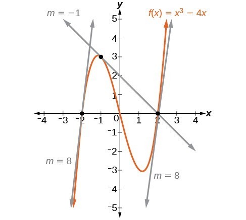
Figure 1

Graph showing tangents to curve at –2, –1, and 2.

Let’s imagine a point on the curve of function [latex]f[/latex] at [latex]x=a[/latex] as shown in Figure 2. The coordinates of the point are [latex]\left(a,f\left(a\right)\right)[/latex]. Connect this point with a second point on the curve a little to the right of [latex]x=a[/latex], with an x-value increased by some small real number [latex]h[/latex]. The coordinates of this second point are [latex]\left(a+h,f\left(a+h\right)\right)[/latex] for some positive-value [latex]h[/latex].

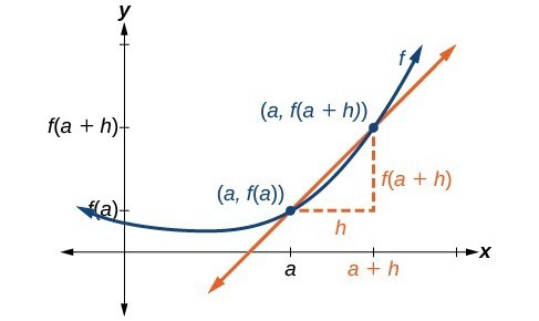
Figure 2. Connecting point [latex]a[/latex] with a point just beyond allows us to measure a slope close to that of a tangent line at [latex]x=a[/latex].

We can calculate the slope of the line connecting the two points [latex]\left(a,f\left(a\right)\right)[/latex] and [latex]\left(a+h,f\left(a+h\right)\right)[/latex], called a secant line, by applying the slope formula,

[latex]\text{slope = }\frac{\text{change in }y}{\text{change in }x}[/latex]

We use the notation [latex]{m}_{\sec }[/latex] to represent the slope of the secant line connecting two points.

The slope [latex]{m}_{\sec }[/latex] equals the average rate of change between two points [latex]\left(a,f\left(a\right)\right)[/latex] and [latex]\left(a+h,f\left(a+h\right)\right)[/latex].

Understanding the Instantaneous Rate of Change

Now that we can find the average rate of change, suppose we make [latex]h[/latex] in Figure 3 smaller and smaller. Then [latex]a+h[/latex] will approach [latex]a[/latex] as [latex]h[/latex] gets smaller, getting closer and closer to 0. Likewise, the second point [latex]\left(a+h,f\left(a+h\right)\right)[/latex] will approach the first point, [latex]\left(a,f\left(a\right)\right)[/latex]. As a consequence, the connecting line between the two points, called the secant line, will get closer and closer to being a tangent to the function at [latex]x=a[/latex], and the slope of the secant line will get closer and closer to the slope of the tangent at [latex]x=a[/latex].

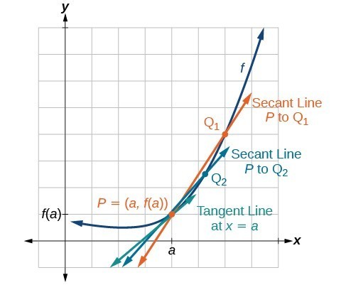
Figure 3

The connecting line between two points moves closer to being a tangent line at [latex]x=a[/latex].

Because we are looking for the slope of the tangent at [latex]x=a[/latex], we can think of the measure of the slope of the curve of a function [latex]f[/latex] at a given point as the rate of change at a particular instant. We call this slope the instantaneous rate of change, or the derivative of the function at [latex]x=a[/latex]. Both can be found by finding the limit of the slope of a line connecting the point at [latex]x=a[/latex] with a second point infinitesimally close along the curve. For a function [latex]f[/latex] both the instantaneous rate of change of the function and the derivative of the function at [latex]x=a[/latex] are written as [latex]f\text{'}\left(a\right)[/latex], and we can define them as a two-sided limit that has the same value whether approached from the left or the right.

The expression by which the limit is found is known as the difference quotient.

The derivative of a function can be interpreted in different ways. It can be observed as the behavior of a graph of the function or calculated as a numerical rate of change of the function.

• The derivative of a function [latex]f\left(x\right)[/latex] at a point [latex]x=a[/latex] is the slope of the tangent line to the curve [latex]f\left(x\right)[/latex] at [latex]x=a[/latex]. The derivative of [latex]f\left(x\right)[/latex] at [latex]x=a[/latex] is written [latex]\begin{align}{f}^{\prime }\left(a\right)\end{align}[/latex].
• The derivative [latex]\begin{align}{f}^{\prime }\left(a\right)\end{align}[/latex] measures how the curve changes at the point [latex]\left(a,f\left(a\right)\right)[/latex].
• The derivative [latex]\begin{align}{f}^{\prime }\left(a\right)\end{align}[/latex] may be thought of as the instantaneous rate of change of the function [latex]f\left(x\right)[/latex] at [latex]x=a[/latex].
• If a function measures distance as a function of time, then the derivative measures the instantaneous velocity at time [latex]t=a[/latex].

Finding Derivatives of Rational Functions

To find the derivative of a rational function, we will sometimes simplify the expression using algebraic techniques we have already learned.

Finding Derivatives of Functions with Roots

To find derivatives of functions with roots, we use the methods we have learned to find limits of functions with roots, including multiplying by a conjugate.

Finding Instantaneous Rates of Change

Many applications of the derivative involve determining the rate of change at a given instant of a function with the independent variable time—which is why the term instantaneous is used. Consider the height of a ball tossed upward with an initial velocity of 64 feet per second, given by [latex]s\left(t\right)=-16{t}^{2}+64t+6[/latex], where [latex]t[/latex] is measured in seconds and [latex]s\left(t\right)[/latex] is measured in feet. We know the path is that of a parabola. The derivative will tell us how the height is changing at any given point in time. The height of the ball is shown in Figure 4 as a function of time. In physics, we call this the “s–t graph.”

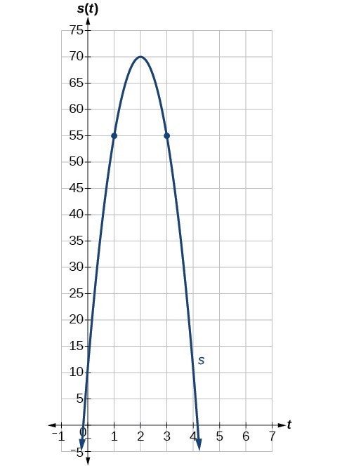
Figure 4

Using Graphs to Find Instantaneous Rates of Change

We can estimate an instantaneous rate of change at [latex]x=a[/latex] by observing the slope of the curve of the function [latex]f\left(x\right)[/latex] at [latex]x=a[/latex]. We do this by drawing a line tangent to the function at [latex]x=a[/latex] and finding its slope.

Example 6: Estimating the Derivative at a Point on the Graph of a Function

From the graph of the function [latex]y=f\left(x\right)[/latex] presented in Figure 5, estimate each of the following:

1. [latex]f\left(0\right)[/latex]
2. [latex]f\left(2\right)[/latex]
3. [latex]\begin{align}f^{\prime}\left(0\right)\end{align}[/latex]
4. [latex]\begin{align}f^{\prime}\left(2\right)\end{align}[/latex]

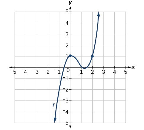
Figure 5

Show Solution

To find the functional value, [latex]f\left(a\right)[/latex], find the y-coordinate at [latex]x=a[/latex].

To find the derivative at [latex]x=a[/latex], [latex]\begin{align}{f}^{\prime }\left(a\right)\end{align}[/latex], draw a tangent line at [latex]x=a[/latex], and estimate the slope of that tangent line.

Figure 6

1. [latex]f\left(0\right)[/latex] is the y-coordinate at [latex]x=0[/latex]. The point has coordinates [latex]\left(0,1\right)[/latex], thus [latex]f\left(0\right)=1[/latex].
2. [latex]f\left(2\right)[/latex] is the y-coordinate at [latex]x=2[/latex]. The point has coordinates [latex]\left(2,1\right)[/latex], thus [latex]f\left(2\right)=1[/latex].
3. [latex]\begin{align}{f}^{\prime }\left(0\right)\end{align}[/latex] is found by estimating the slope of the tangent line to the curve at [latex]x=0[/latex]. The tangent line to the curve at [latex]x=0[/latex] appears horizontal. Horizontal lines have a slope of 0, thus [latex]{f}^{\prime }\left(0\right)=0[/latex].
4. [latex]\begin{align}{f}^{\prime }\left(2\right)\end{align}[/latex] is found by estimating the slope of the tangent line to the curve at [latex]x=2[/latex]. Observe the path of the tangent line to the curve at [latex]x=2[/latex]. As the [latex]x[/latex] value moves one unit to the right, the [latex]y[/latex] value moves up four units to another point on the line. Thus, the slope is 4, so [latex]\begin{align}{f}^{\prime }\left(2\right)\end{align}=4[/latex].

Try It

Using the graph of the function [latex]f\left(x\right)={x}^{3}-3x[/latex] shown in Figure 7, estimate: [latex]f\left(1\right)[/latex], [latex]\begin{align}{f}^{\prime }\left(1\right)\end{align}[/latex], [latex]f\left(0\right)[/latex], and [latex]\begin{align}{f}^{\prime }\left(0\right)\end{align}[/latex].

Figure 7

Show Solution

[latex]-2,0,0,-3[/latex]

Using Instantaneous Rates of Change to Solve Real-World Problems

Another way to interpret an instantaneous rate of change at [latex]x=a[/latex] is to observe the function in a real-world context. The unit for the derivative of a function [latex]f\left(x\right)[/latex] is

Such a unit shows by how many units the output changes for each one-unit change of input. The instantaneous rate of change at a given instant shows the same thing: the units of change of output per one-unit change of input.

One example of an instantaneous rate of change is a marginal cost. For example, suppose the production cost for a company to produce [latex]x[/latex] items is given by [latex]C\left(x\right)[/latex], in thousands of dollars. The derivative function tells us how the cost is changing for any value of [latex]x[/latex] in the domain of the function. In other words, [latex]\begin{align}{C}^{\prime }\left(x\right)\end{align}[/latex] is interpreted as a marginal cost, the additional cost in thousands of dollars of producing one more item when [latex]x[/latex] items have been produced. For example, [latex]\begin{align}{C}^{\prime }\left(11\right)\end{align}[/latex] is the approximate additional cost in thousands of dollars of producing the 12^th item after 11 items have been produced. [latex]\begin{align}{C}^{\prime }\left(11\right)=2.50\end{align}[/latex] means that when 11 items have been produced, producing the 12^th item would increase the total cost by approximately $2,500.00.

Finding Points Where a Function’s Derivative Does Not Exist

To understand where a function’s derivative does not exist, we need to recall what normally happens when a function [latex]f\left(x\right)[/latex] has a derivative at [latex]x=a[/latex] . Suppose we use a graphing utility to zoom in on [latex]x=a[/latex] . If the function [latex]f\left(x\right)[/latex] is differentiable, that is, if it is a function that can be differentiated, then the closer one zooms in, the more closely the graph approaches a straight line. This characteristic is called linearity.

Look at the graph in Figure 8. The closer we zoom in on the point, the more linear the curve appears.

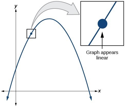
Figure 8

We might presume the same thing would happen with any continuous function, but that is not so. The function [latex]f\left(x\right)=|x|[/latex], for example, is continuous at [latex]x=0[/latex], but not differentiable at [latex]x=0[/latex]. As we zoom in close to 0 in Figure 9, the graph does not approach a straight line. No matter how close we zoom in, the graph maintains its sharp corner.

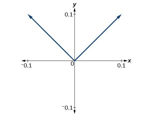
Figure 9. Graph of the function [latex]f\left(x\right)=|x|[/latex], with x-axis from –0.1 to 0.1 and y-axis from –0.1 to 0.1.

We zoom in closer by narrowing the range to produce Figure 10 and continue to observe the same shape. This graph does not appear linear at [latex]x=0[/latex].

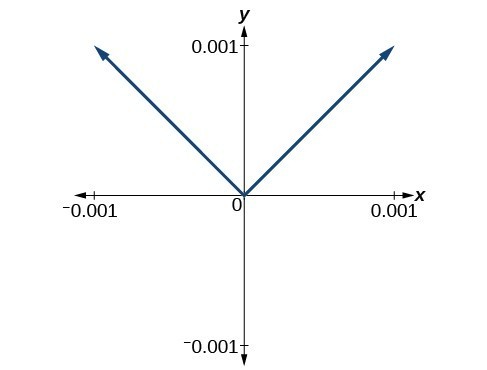
Figure 10. Graph of the function [latex]f\left(x\right)=|x|[/latex], with x-axis from –0.001 to 0.001 and y-axis from—0.001 to 0.001.

What are the characteristics of a graph that is not differentiable at a point? Here are some examples in which function [latex]f\left(x\right)[/latex] is not differentiable at [latex]x=a[/latex].

In Figure 11, we see the graph of

[latex]f\left(x\right)=\begin{cases}x^{2}, \hfill& x\leq 2 \\ 8-x, \hfill& x>2\end{cases}[/latex].

Notice that, as [latex]x[/latex] approaches 2 from the left, the left-hand limit may be observed to be 4, while as [latex]x[/latex] approaches 2 from the right, the right-hand limit may be observed to be 6. We see that it has a discontinuity at [latex]x=2[/latex].

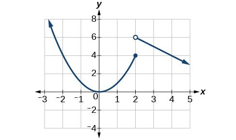
Figure 11

The graph of [latex]f\left(x\right)[/latex] has a discontinuity at [latex]x=2[/latex].

In Figure 12, we see the graph of [latex]f\left(x\right)=|x|[/latex]. We see that the graph has a corner point at [latex]x=0[/latex].

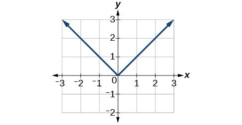
Figure 12. The graph of [latex]f\left(x\right)=|x|[/latex] has a corner point at [latex]x=0[/latex] .

The graph of [latex]f\left(x\right)=|x|[/latex] has a corner point at [latex]x=0[/latex] .

In Figure 13, we see that the graph of [latex]f\left(x\right)={x}^{\frac{2}{3}}[/latex] has a cusp at [latex]x=0[/latex]. A cusp has a unique feature. Moving away from the cusp, both the left-hand and right-hand limits approach either infinity or negative infinity. Notice the tangent lines as [latex]x[/latex] approaches 0 from both the left and the right appear to get increasingly steeper, but one has a negative slope, the other has a positive slope.

Figure 13. The graph of [latex]f\left(x\right)={x}^{\frac{2}{3}}[/latex] has a cusp at [latex]x=0[/latex].

In Figure 14, we see that the graph of [latex]f\left(x\right)={x}^{\frac{1}{3}}[/latex] has a vertical tangent at [latex]x=0[/latex]. Recall that vertical tangents are vertical lines, so where a vertical tangent exists, the slope of the line is undefined. This is why the derivative, which measures the slope, does not exist there.

Figure 14. The graph of [latex]f\left(x\right)={x}^{\frac{1}{3}}[/latex] has a vertical tangent at [latex]x=0[/latex].

Example 9: Determining Where a Function Is Continuous and Differentiable from a Graph

Using Figure 15, determine where the function is

1. continuous
2. discontinuous
3. differentiable
4. not differentiable

At the points where the graph is discontinuous or not differentiable, state why.

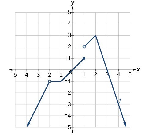
Figure 15

Show Solution

The graph of [latex]f\left(x\right)[/latex] is continuous on [latex]\left(\mathrm{-\infty ,}-2\right)\cup \left(-2, 1\right)\cup \left(1,\infty \right)[/latex]. The graph of [latex]f\left(x\right)[/latex] has a removable discontinuity at [latex]x=-2[/latex] and a jump discontinuity at [latex]x=1[/latex].

Figure 16. Three intervals where the function is continuous

The graph of is differentiable on [latex]\left(\mathrm{-\infty ,}-2\right)\cup \left(-2,-1\right)\cup \left(-1,1\right)\cup \left(1,2\right)\cup \left(2,\infty \right)[/latex]. The graph of [latex]f\left(x\right)[/latex] is not differentiable at [latex]x=-2[/latex] because it is a point of discontinuity, at [latex]x=-1[/latex] because of a sharp corner, at [latex]x=1[/latex] because it is a point of discontinuity, and at [latex]x=2[/latex] because of a sharp corner.

Figure 17. Five intervals where the function is differentiable

Try It

Determine where the function [latex]y=f\left(x\right)[/latex] shown in Figure 18 is continuous and differentiable from the graph.

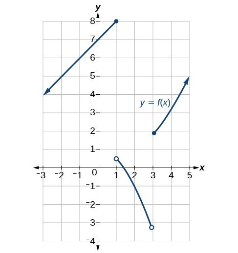
Figure 18

Show Solution

The graph of [latex]f[/latex] is continuous on [latex]\left(-\infty ,1\right)\cup \left(1,3\right)\cup \left(3,\infty \right)[/latex]. The graph of [latex]f[/latex] is discontinuous at [latex]x=1[/latex] and [latex]x=3[/latex]. The graph of [latex]f[/latex] is differentiable on [latex]\left(-\infty ,1\right)\cup \left(1,3\right)\cup \left(3,\infty \right)[/latex]. The graph of [latex]f[/latex] is not differentiable at [latex]x=1[/latex] and [latex]x=3[/latex].

Finding an Equation of a Line Tangent to the Graph of a Function

The equation of a tangent line to a curve of the function [latex]f\left(x\right)[/latex] at [latex]x=a[/latex] is derived from the point-slope form of a line, [latex]y=m\left(x-{x}_{1}\right)+{y}_{1}[/latex]. The slope of the line is the slope of the curve at [latex]x=a[/latex] and is therefore equal to [latex]\begin{align}{f}^{\prime }\left(a\right)\end{align}[/latex], the derivative of [latex]f\left(x\right)[/latex] at [latex]x=a[/latex]. The coordinate pair of the point on the line at [latex]x=a[/latex] is [latex]\left(a,f\left(a\right)\right)[/latex].

If we substitute into the point-slope form, we have

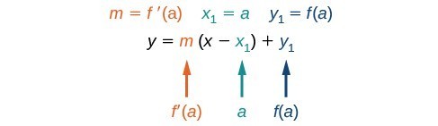
The equation of the tangent line is

Example 10: Finding the Equation of a Line Tangent to a Function at a Point

Find the equation of a line tangent to the curve [latex]f\left(x\right)={x}^{2}-4x[/latex] at [latex]x=3[/latex].

Show Solution

Using:

[latex]f^{\prime}\left(a\right)=\underset{h\to 0}{\mathrm{lim}}\frac{f\left(a+h\right)-f\left(a\right)}{h}[/latex]

Substitute [latex]f\left(a+h\right)={\left(a+h\right)}^{2}-4\left(a+h\right)[/latex] and [latex]f\left(a\right)={a}^{2}-4a[/latex].

[latex]\begin{align} {f}^{\prime }\left(a\right)&=\underset{h\to 0}{\mathrm{lim}}\frac{\left(a+h\right)\left(a+h\right)-4\left(a+h\right)-\left({a}^{2}-4a\right)}{h} \\ &=\underset{h\to 0}{\mathrm{lim}}\frac{{a}^{2}+2ah+{h}^{2}-4a - 4h-{a}^{2}+4a}{h}&& \text{Remove parentheses}. \\ &=\underset{h\to 0}{\mathrm{lim}}\frac{{a}^{2}+2ah+{h}^{2}-4a-4h-{a}^{2}+4a}{h}&& \text{Combine like terms}. \\ &=\underset{h\to 0}{\mathrm{lim}}\frac{2ah+{h}^{2}-4h}{h} \\ &=\underset{h\to 0}{\mathrm{lim}}\frac{\cancel{h}\left(2a+h - 4\right)}{\cancel{h}}&& \text{Factor out }h. \\ &=2a+0 - 4 \\ {f}^{\prime }\left(a\right)&=2a - 4&& \text{Evaluate the limit}. \\ {f}^{\prime }\left(3\right)&=2\left(3\right)-4=2 \end{align}[/latex]

Equation of tangent line at [latex]x=3:[/latex]

[latex]\begin{align}&y=f^{\prime}\left(a\right)\left(x-a\right)+f\left(a\right) \\ &y=f^{\prime}\left(3\right)\left(x - 3\right)+f\left(3\right) \\ &y=2\left(x - 3\right)+\left(-3\right) \\ &y=2x - 9 \end{align}[/latex]

Analysis of the Solution

We can use a graphing utility to graph the function and the tangent line. In so doing, we can observe the point of tangency at [latex]x=3[/latex] as shown in Figure 19.

Figure 19. Graph confirms the point of tangency at [latex]x=3[/latex].

Finding the Instantaneous Speed of a Particle

If a function measures position versus time, the derivative measures displacement versus time, or the speed of the object. A change in speed or direction relative to a change in time is known as velocity. The velocity at a given instant is known as instantaneous velocity.

In trying to find the speed or velocity of an object at a given instant, we seem to encounter a contradiction. We normally define speed as the distance traveled divided by the elapsed time. But in an instant, no distance is traveled, and no time elapses. How will we divide zero by zero? The use of a derivative solves this problem. A derivative allows us to say that even while the object’s velocity is constantly changing, it has a certain velocity at a given instant. That means that if the object traveled at that exact velocity for a unit of time, it would travel the specified distance.

Key Equations

Key Concepts

• The slope of the secant line connecting two points is the average rate of change of the function between those points.
• The derivative, or instantaneous rate of change, is a measure of the slope of the curve of a function at a given point, or the slope of the line tangent to the curve at that point.
• The difference quotient is the quotient in the formula for the instantaneous rate of change:

  [latex]\frac{f\left(a+h\right)-f\left(a\right)}{h}[/latex]

• Instantaneous rates of change can be used to find solutions to many real-world problems.
• The instantaneous rate of change can be found by observing the slope of a function at a point on a graph by drawing a line tangent to the function at that point.
• Instantaneous rates of change can be interpreted to describe real-world situations.
• Some functions are not differentiable at a point or points.
• The point-slope form of a line can be used to find the equation of a line tangent to the curve of a function.
• Velocity is a change in position relative to time. Instantaneous velocity describes the velocity of an object at a given instant. Average velocity describes the velocity maintained over an interval of time.
• Using the derivative makes it possible to calculate instantaneous velocity even though there is no elapsed time.

Glossary

average rate of change

the slope of the line connecting the two points [latex]\left(a,f\left(a\right)\right)[/latex] and [latex]\left(a+h,f\left(a+h\right)\right)[/latex] on the curve of [latex]f\left(x\right)[/latex]; it is given by [latex]\text{AROC}=\frac{f\left(a+h\right)-f\left(a\right)}{h}[/latex].

derivative

the slope of a function at a given point; denoted [latex]\begin{align}{f}^{\prime }\left(a\right)\end{align}[/latex], at a point [latex]x=a[/latex] it is [latex]{f}^{\prime }\left(a\right)=\underset{h\to 0}{\mathrm{lim}}\dfrac{f\left(a+h\right)-f\left(a\right)}{h}[/latex], providing the limit exists.

differentiable

a function [latex]f\left(x\right)[/latex] for which the derivative exists at [latex]x=a[/latex]. In other words, if [latex]\begin{align}{f}^{\prime }\left(a\right)\end{align}[/latex] exists.

instantaneous rate of change

the slope of a function at a given point; at [latex]x=a[/latex] it is given by [latex]{f}^{\prime }\left(a\right)=\underset{h\to 0}{\mathrm{lim}}\dfrac{f\left(a+h\right)-f\left(a\right)}{h}[/latex].

instantaneous velocity

the change in speed or direction at a given instant; a function [latex]s\left(t\right)[/latex] represents the position of an object at time [latex]t[/latex], and the instantaneous velocity or velocity of the object at time [latex]t=a[/latex] is given by [latex]{s}^{\prime }\left(a\right)=\underset{h\to 0}{\mathrm{lim}}\dfrac{s\left(a+h\right)-s\left(a\right)}{h}[/latex].

secant line

a line that intersects two points on a curve

tangent line

a line that intersects a curve at a single point