Learning Outcomes
- Solve direct variation problems.
- Solve inverse variation problems.
- Solve problems involving joint variation.
A used-car company has just offered their best candidate, Nicole, a position in sales. The position offers 16% commission on her sales. Her earnings depend on the amount of her sales. For instance, if she sells a vehicle for $4,600, she will earn $736. She wants to evaluate the offer, but she is not sure how. In this section, we will look at relationships, such as this one, between earnings, sales, and commission rate.
Solve direct variation problems
In the example above, Nicole’s earnings can be found by multiplying her sales by her commission. The formula e = 0.16s tells us her earnings, e, come from the product of 0.16, her commission, and the sale price of the vehicle. If we create a table, we observe that as the sales price increases, the earnings increase as well, which should be intuitive.
| s, sales prices | e = 0.16s | Interpretation |
|---|---|---|
| $4,600 | e = 0.16(4,600) = 736 | A sale of a $4,600 vehicle results in $736 earnings. |
| $9,200 | e = 0.16(9,200) = 1,472 | A sale of a $9,200 vehicle results in $1472 earnings. |
| $18,400 | e = 0.16(18,400) = 2,944 | A sale of a $18,400 vehicle results in $2944 earnings. |
Notice that earnings are a multiple of sales. As sales increase, earnings increase in a predictable way. Double the sales of the vehicle from $4,600 to $9,200, and we double the earnings from $736 to $1,472. As the input increases, the output increases as a multiple of the input. A relationship in which one quantity is a constant multiplied by another quantity is called direct variation. Each variable in this type of relationship varies directly with the other.
The graph below represents the data for Nicole’s potential earnings. We say that earnings vary directly with the sales price of the car. The formula [latex]y=k{x}^{n}[/latex] is used for direct variation. The value k is a nonzero constant greater than zero and is called the constant of variation. In this case, k = 0.16 and n = 1.
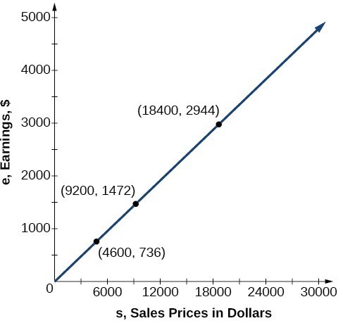
Figure 1
A General Note: Direct Variation
If x and y are related by an equation of the form
then we say that the relationship is direct variation and y varies directly with the nth power of x. In direct variation relationships, there is a nonzero constant ratio [latex]k=\frac{y}{{x}^{n}}[/latex], where k is called the constant of variation, which help defines the relationship between the variables.
How To: Given a description of a direct variation problem, solve for an unknown.
- Identify the input, x, and the output, y.
- Determine the constant of variation. You may need to divide y by the specified power of x to determine the constant of variation.
- Use the constant of variation to write an equation for the relationship.
- Substitute known values into the equation to find the unknown.
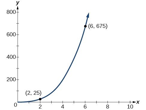
Example 1: Solving a Direct Variation Problem
The quantity y varies directly with the cube of x. If y = 25 when x = 2, find y when x is 6.
Q & A
Do the graphs of all direct variation equations look like Example 1?
No. Direct variation equations are power functions—they may be linear, quadratic, cubic, quartic, radical, etc. But all of the graphs pass through (0, 0).
Try It
The quantity y varies directly with the square of x. If y = 24 when x = 3, find y when x is 4.
Try It
Solve inverse variation problems
Water temperature in an ocean varies inversely to the water’s depth. Between the depths of 250 feet and 500 feet, the formula [latex]T=\frac{14,000}{d}[/latex] gives us the temperature in degrees Fahrenheit at a depth in feet below Earth’s surface. Consider the Atlantic Ocean, which covers 22% of Earth’s surface. At a certain location, at the depth of 500 feet, the temperature may be 28°F.
If we create a table we observe that, as the depth increases, the water temperature decreases.
| d, depth | [latex]T=\frac{\text{14,000}}{d}[/latex] | Interpretation |
|---|---|---|
| 500 ft | [latex]\frac{14,000}{500}=28[/latex] | At a depth of 500 ft, the water temperature is 28° F. |
| 350 ft | [latex]\frac{14,000}{350}=40[/latex] | At a depth of 350 ft, the water temperature is 40° F. |
| 250 ft | [latex]\frac{14,000}{250}=56[/latex] | At a depth of 250 ft, the water temperature is 56° F. |
We notice in the relationship between these variables that, as one quantity increases, the other decreases. The two quantities are said to be inversely proportional and each term varies inversely with the other. Inversely proportional relationships are also called inverse variations.
For our example, the graph depicts the inverse variation. We say the water temperature varies inversely with the depth of the water because, as the depth increases, the temperature decreases. The formula [latex]y=\frac{k}{x}[/latex] for inverse variation in this case uses k = 14,000.
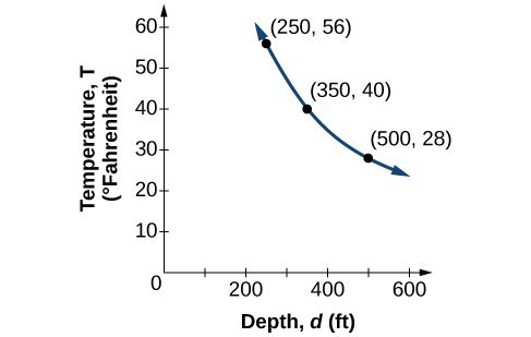
Figure 3
A General Note: Inverse Variation
If x and y are related by an equation of the form
where k is a nonzero constant, then we say that y varies inversely with the nth power of x. In inversely proportional relationships, or inverse variations, there is a constant multiple [latex]k={x}^{n}y[/latex].
Example 2: Writing a Formula for an Inversely Proportional Relationship
A tourist plans to drive 100 miles. Find a formula for the time the trip will take as a function of the speed the tourist drives.
How To: Given a description of an indirect variation problem, solve for an unknown.
- Identify the input, x, and the output, y.
- Determine the constant of variation. You may need to multiply y by the specified power of x to determine the constant of variation.
- Use the constant of variation to write an equation for the relationship.
- Substitute known values into the equation to find the unknown.
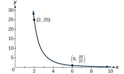
Example 3: Solving an Inverse Variation Problem
A quantity y varies inversely with the cube of x. If y = 25 when x = 2, find y when x is 6.
Try It
A quantity y varies inversely with the square of x. If y = 8 when x = 3, find y when x is 4.
Try It
Solve problems involving joint variation
Many situations are more complicated than a basic direct variation or inverse variation model. One variable often depends on multiple other variables. When a variable is dependent on the product or quotient of two or more variables, this is called joint variation. For example, the cost of busing students for each school trip varies with the number of students attending and the distance from the school. The variable c, cost, varies jointly with the number of students, n, and the distance, d.
A General Note: Joint Variation
Joint variation occurs when a variable varies directly or inversely with multiple variables.
For instance, if x varies directly with both y and z, we have x = kyz. If x varies directly with y and inversely with z, we have [latex]x=\frac{ky}{z}[/latex]. Notice that we only use one constant in a joint variation equation.
Example 4: Solving Problems Involving Joint Variation
A quantity x varies directly with the square of y and inversely with the cube root of z. If x = 6 when y = 2 and z = 8, find x when y = 1 and z = 27.
Try It
x varies directly with the square of y and inversely with z. If x = 40 when y = 4 and z = 2, find x when y = 10 and z = 25.
Key Takeaways
Key Equations
| Direct variation | [latex]y=k{x}^{n},k\text{ is a nonzero constant}[/latex]. |
| Inverse variation | [latex]y=\frac{k}{{x}^{n}},k\text{ is a nonzero constant}[/latex]. |
Key Concepts
- A relationship where one quantity is a constant multiplied by another quantity is called direct variation.
- Two variables that are directly proportional to one another will have a constant ratio.
- A relationship where one quantity is a constant divided by another quantity is called inverse variation.
- Two variables that are inversely proportional to one another will have a constant multiple.
- In many problems, a variable varies directly or inversely with multiple variables. We call this type of relationship joint variation.
Glossary
- constant of variation
- the non-zero value k that helps define the relationship between variables in direct or inverse variation
- direct variation
- the relationship between two variables that are a constant multiple of each other; as one quantity increases, so does the other
- inverse variation
- the relationship between two variables in which the product of the variables is a constant
- inversely proportional
- a relationship where one quantity is a constant divided by the other quantity; as one quantity increases, the other decreases
- joint variation
- a relationship where a variable varies directly or inversely with multiple variables
- varies directly
- a relationship where one quantity is a constant multiplied by the other quantity
- varies inversely
- a relationship where one quantity is a constant divided by the other quantity
Candela Citations
- Precalculus. Authored by: OpenStax College. Provided by: OpenStax. Located at: http://cnx.org/contents/fd53eae1-fa23-47c7-bb1b-972349835c3c@5.175:1/Preface. License: CC BY: Attribution