Identifying ordered pairs as solutions to linear equations

A line is a visual representation of a linear equation, and the line itself is made up of an infinite number of points (or ordered pairs). The picture below shows the line of the linear equation [latex]y=2x–5[/latex] with some of the specific points on the line.

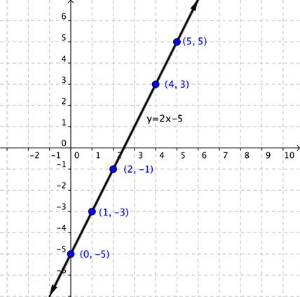
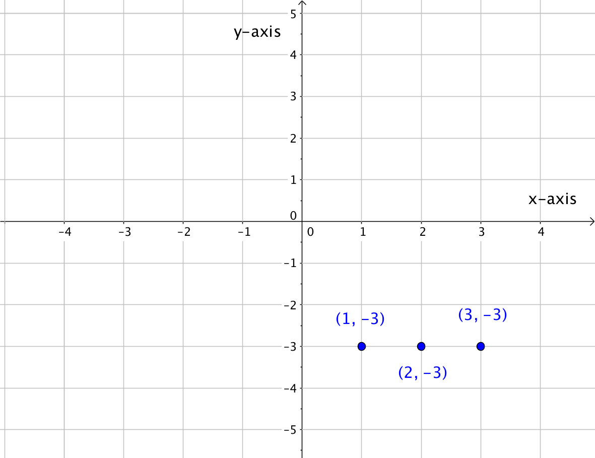
Every point on the line is a solution to the equation [latex]y=2x–5[/latex]. You can try plugging in any of the points that are labeled, like the ordered pair, [latex](1,−3)[/latex].

[latex]\begin{array}{l}\,\,\,\,y=2x-5\\-3=2\left(1\right)-5\\-3=2-5\\-3=-3\\\text{This is true.}\end{array}[/latex]

You can also try ANY of the other points on the line. Every point on the line is a solution to the equation [latex]y=2x–5[/latex]. All this means is that determining whether an ordered pair is a solution of an equation is pretty straightforward. If the ordered pair is on the line created by the linear equation, then it is a solution to the equation. But if the ordered pair is not on the line—no matter how close it may look—then it is not a solution to the equation.

Graphing lines using ordered pairs

Graphing ordered pairs helps us make sense of all kinds of mathematical relationships.

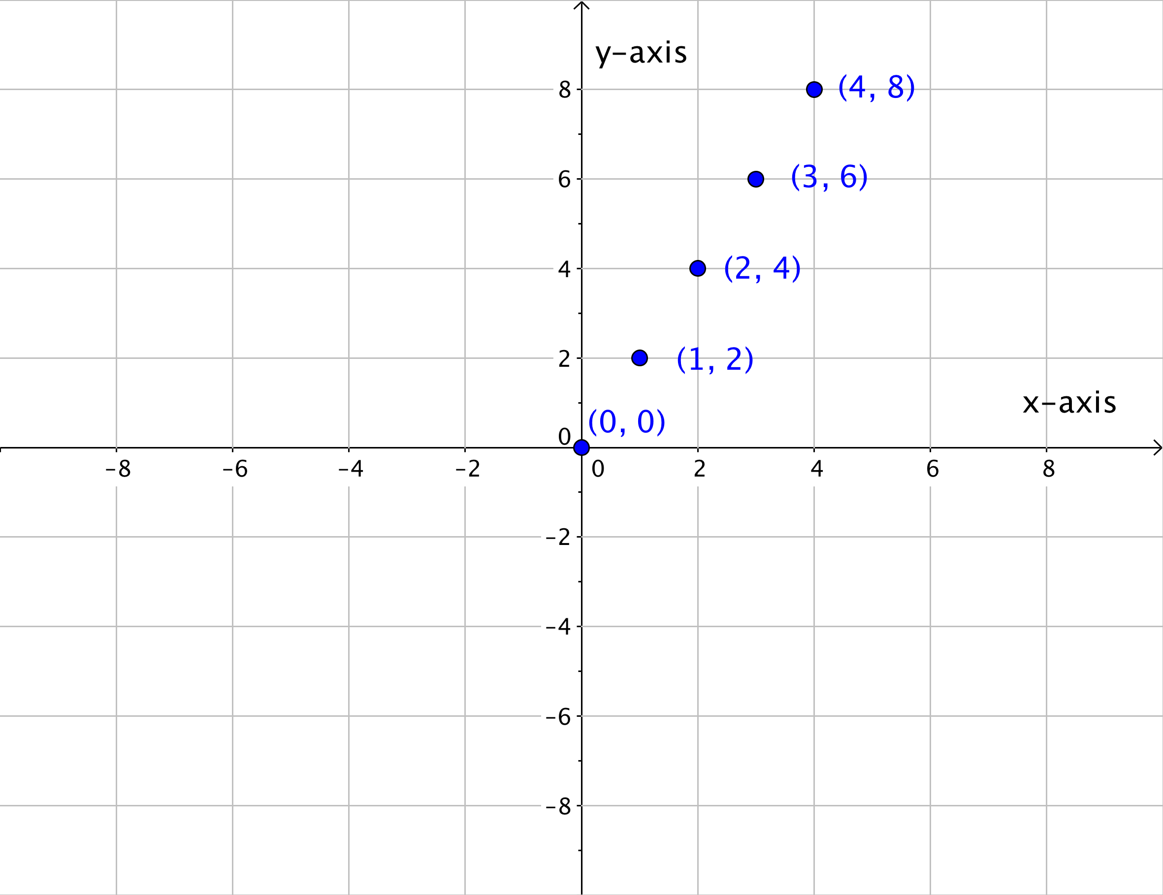
A linear relationship is a relationship between variables such that when plotted on a coordinate plane, the points lie on a line. Let’s start by looking at a series of points in Quadrant I on the coordinate plane.

Look at the five ordered pairs (and their x– and y-coordinates) below. Do you see any pattern to the location of the points? If this pattern continued, what other points could be included?

(0,0) , (1,2) , (2,4) , (3,6) , (4, 8) , (?, ?)

You may have identified that if this pattern continued the next ordered pair would be at (5, 10).  Applying the same logic, you may identify that the ordered pairs (6, 12) and (7, 14) would also belong (if this coordinate plane were larger).

These series of points can also be represented in a table. In the table below, the x- and y-coordinates of each ordered pair on the graph is recorded.

Notice that each y-coordinate is twice the corresponding x-value. All of these x- and y-values follow the same pattern, and, when placed on a coordinate plane, they all line up!

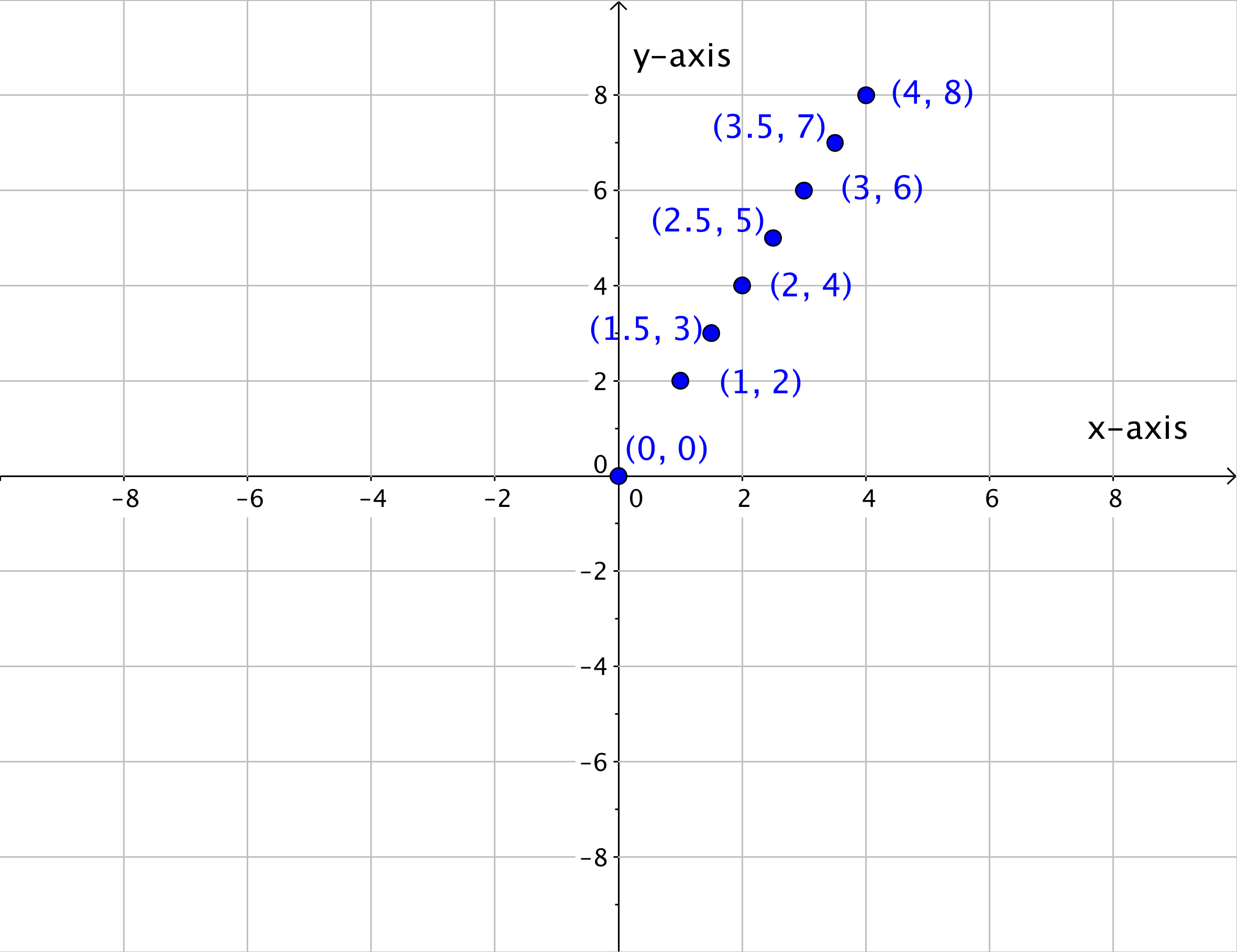
Once you know the pattern that relates the x- and y-values, you can find a y-value for any x-value that lies on the line. So if the rule of this pattern is that each y-value is twice the corresponding x-value, then the ordered pairs (1.5, 3), (2.5, 5), and (3.5, 7) should all appear on the line too, correct? Look to see what happens.

If you were to keep adding ordered pairs (x, y) where the y-value was twice the x-value, you would end up with a graph like this.

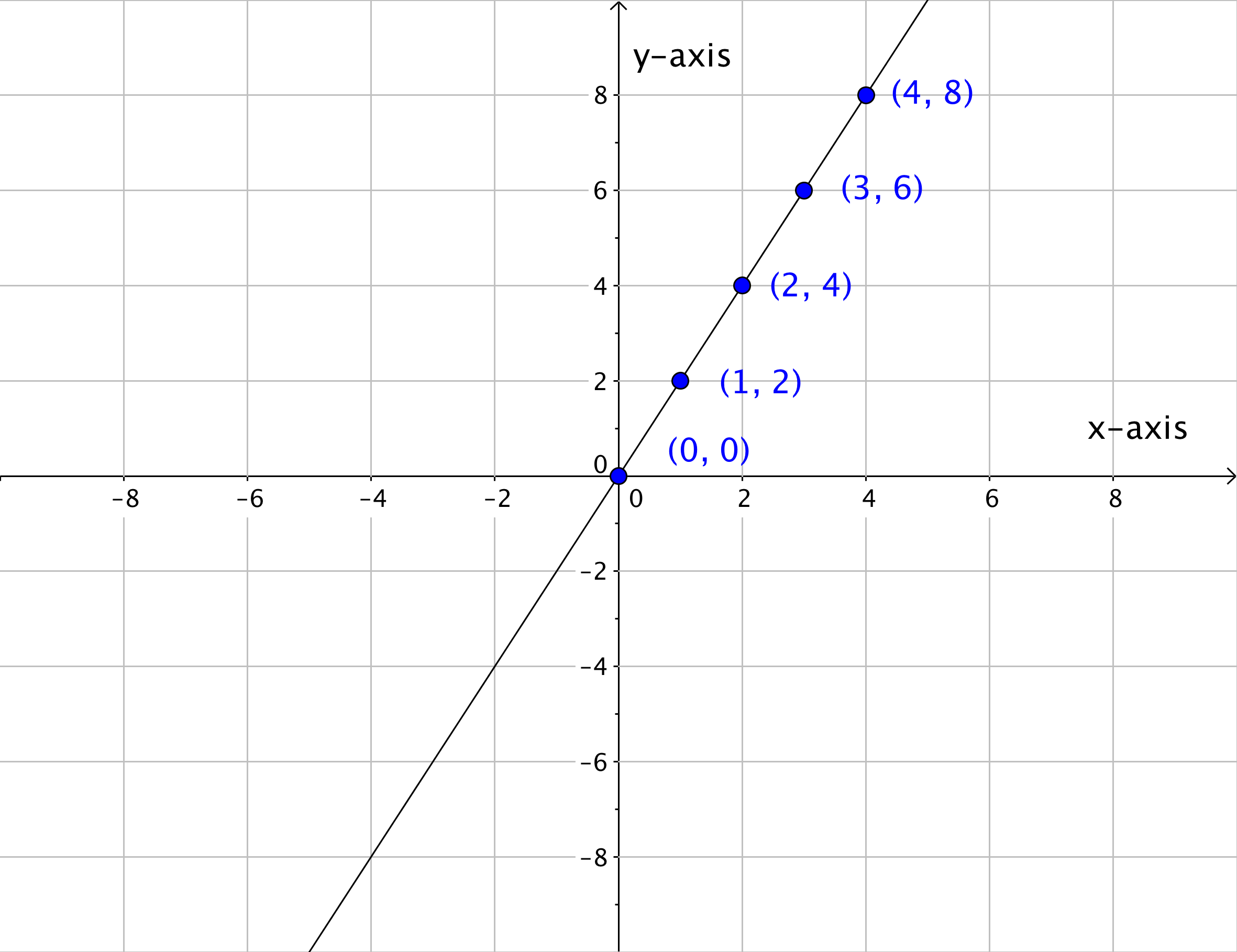
Look at how all of the points blend together to create a line. You can think of a line, then, as a collection of an infinite number of individual points that share the same mathematical relationship. In this case, the relationship is that the y-value is twice the x-value.

There are multiple ways to represent a linear relationship—a table, a linear graph, and there is also a linear equation. A linear equation is an equation with two variables whose ordered pairs graph as a straight line.

There are several ways to create a graph from a linear equation. One way is to create a table of values for x and y, and then plot these ordered pairs on the coordinate plane. Two points are enough to determine a line. However, it’s always a good idea to plot more than two points to avoid possible errors.

Then you draw a line through the points to show all of the points that are on the line. The line continues endlessly in both directions. Every point on this line is a solution to the linear equation.

Example 3

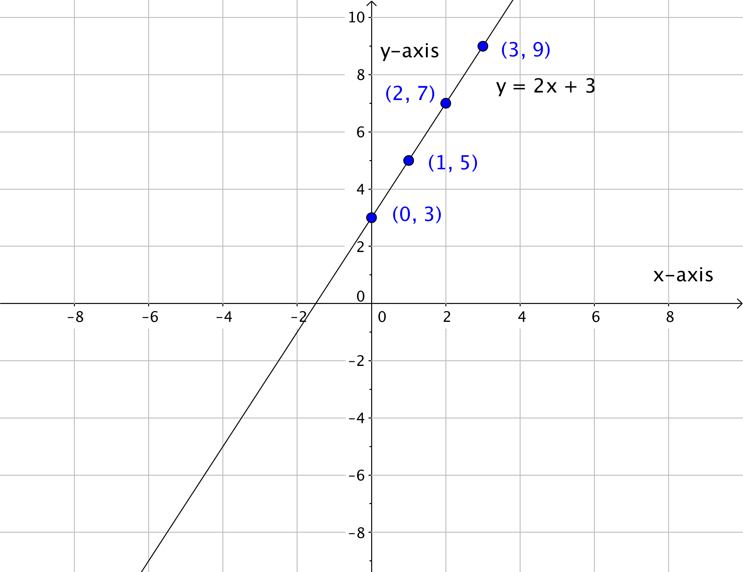
Graph the linear equation [latex]y=2x+3[/latex].

Show Solution

Evaluate [latex]y=2x+3[/latex] for different values of x, and create a table of corresponding x and y values.

x values	[latex]2x+3[/latex]	y values
0	[latex]2(0) + 3[/latex]	3
1	[latex]2(1) + 3[/latex]	5
2	[latex]2(2) + 3[/latex]	7
3	[latex]2(3) + 3[/latex]	9

Convert the table to ordered pairs. Plot the ordered pairs.

[latex](0, 3)[/latex]

[latex](1, 5)[/latex]

[latex](2, 7)[/latex]

[latex](3, 9)[/latex]

 

Draw a line through the points to indicate all of the points on the line.

Answer

Identify the intercepts of a linear equation

The intercepts of a line are the points where the line intersects, or crosses, the horizontal and vertical axes. To help you remember what “intercept” means, think about the word “intersect.” The two words sound alike and in this case mean the same thing.

The straight line on the graph below intersects the two coordinate axes. The point where the line crosses the x-axis is called the x-intercept. The y-intercept is the point where the line crosses the y-axis.

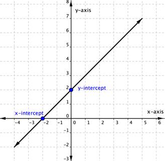
The x-intercept above is the point [latex](−2,0)[/latex]. The y-intercept above is the point (0, 2).

Notice that the y-intercept always occurs where [latex]x=0[/latex], and the x-intercept always occurs where [latex]y=0[/latex].

To find the x– and y-intercepts of a linear equation, you can substitute 0 for y and for x, respectively.

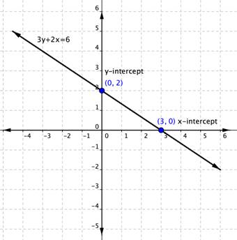
For example, the linear equation [latex]3y+2x=6[/latex] has an x intercept when [latex]y=0[/latex], so [latex]3\left(0\right)+2x=6\\[/latex].

[latex]\begin{array}{r}2x=6\\x=3\end{array}[/latex]

The x-intercept is [latex](3,0)[/latex].

Likewise the y-intercept occurs when [latex]x=0[/latex].

[latex]\begin{array}{r}3y+2\left(0\right)=6\\3y=6\\y=2\end{array}[/latex]

The y-intercept is [latex](0,2)[/latex].

Use the intercepts to graph a linear equation

You can use intercepts to graph some linear equations. Once you have found the two intercepts, draw a line through them.  This method is often used when the equation is written in Standard Form.

Standard Form of a Line

One way that we can represent the equation of a line is in standard form. Standard form is given as

[latex]Ax+By=C[/latex]

where [latex]A[/latex], [latex]B[/latex], and [latex]C[/latex] are integers. The x and y terms are on one side of the equal sign, and the constant term is on the other side.

Let’s use the intercepts to graph the equation [latex]3y+2x=6[/latex]. You figured out that the intercepts of the line this equation represents are [latex](0,2)[/latex] and [latex](3,0)[/latex]. That’s all you need to know.

Example 4

Graph [latex]3x+5y=30[/latex] using the x and y-intercepts.

Show Solution

When an equation is in [latex]Ax+By=C[/latex] form, you can easily find the x– and y-intercepts and then graph.

[latex]\begin{array}{r}3x+5y=30\\3\left(0\right)+5y=30\\0+5y=30\\5y=30\\y=\,\,\,6\\y\text{-intercept}\,\left(0,6\right)\end{array}[/latex]

To find the y-intercept, set [latex]x=0[/latex] and solve for y.

[latex]\begin{array}{r}3x+5y=30\\3x+5\left(0\right)=30\\3x+0=30\\3x=30\\x=10\\x\text{-intercept}\left(10,0\right)\end{array}[/latex]

To find the x-intercept, set [latex]y=0[/latex] and solve for x.

Answer

As we saw in the previous example, when given an equation in the form [latex]Ax+By=C[/latex], it is often easy to find the x and y-intercepts. Note that because of the communitive property of addition, [latex]Ax+By=C[/latex] is equivalent to [latex]By+Ax=C[/latex]. In the example below you will see an example where the equation is in the form [latex]By+Ax=C[/latex].

In the example below, the equation wasn’t given in the form [latex]Ax + By=C[/latex], but we can still find the x and y-intercepts in the form it is in.

Example 5

Graph [latex]y=2x-4[/latex] using the x and y-intercepts.

Show Solution

First, find the y-intercept. Set x equal to zero and solve for y.

[latex]\begin{array}{l}y=2x-4\\y=2\left(0\right)-4\\y=0-4\\y=-4\\y\text{-intercept}\left(0,-4\right)\end{array}[/latex]

To find the x-intercept, set [latex]y=0[/latex] and solve for x.

[latex]\begin{array}{l}y=2x-4\\0=2x-4\\4=2x\\x=2\\x\text{-intercept}\left(2,0\right)\end{array}[/latex]

Answer

We mentioned that we can graph some linear equations using intercepts.  So, what is the exception.  In the next example, there is only one intercept; yet, we need two points to construct a graph!

Example 6

Find the [latex]x[/latex] and [latex]y[/latex]-intercepts and sketch the graph.

[latex]2x-y=0[/latex]

Show Solution

First we find the [latex]y[/latex]-intercept by plugging in [latex]x=0[/latex].

[latex]2(0)-y=0[/latex]

[latex]\frac{-y}{-1}=\frac{0}{-1}[/latex]

[latex]y=0[/latex]

Therefore, the [latex]y[/latex]-intercept is the origin, [latex](0,0)[/latex]

Next, we find the [latex]x[/latex]-intercept by plugging in [latex]y=0[/latex].

[latex]2x-0=0[/latex]

[latex]\frac{2x}{2}=\frac{0}{2}[/latex]

[latex]x=0[/latex]

Hence, the [latex]x[/latex]-intercept is also [latex](0,0)[/latex].

But since this only produces one point on the graph, we will be unable to graph it using intercepts alone.  Instead, we can revert back to plugging in a different value for [latex]x[/latex] (or for [latex]y[/latex]) to find a second solution.

Suppose we plug in [latex]x=1[/latex]. We get

[latex]2(1)-y=0[/latex]

[latex]2-y=0[/latex]

[latex]\underline{-2\hspace{.35in}-2}\hspace{.1in}[/latex]

[latex]\frac{-y}{-1}=\frac{-2}{-1}[/latex]

[latex]y=2[/latex]

So, a second point on the graph is [latex](1,2)[/latex].  Of course, we can continue to find more solutions if we want, but two will be sufficient to produce the graph shown below.

Solve for y, then graph a linear equation

Often times, it is easier to make a table of values if the equation is in the form [latex]y=mx+b[/latex] where m and b are real numbers. But to take advantage of this, we often must first solve for [latex]y[/latex] in the equation.

Example 7

Solve for [latex]y[/latex] and graph using a table of values.

[latex]3x+y=5[/latex].

Show Solution

First, isolate [latex]y[/latex] by subtracting [latex]3x[/latex] on both sides of the equation.

[latex]3x+y=5[/latex]

[latex]\hspace{.02in}\underline{-3x\hspace{.35in}-3x}[/latex]

[latex]y=-3x+5[/latex]

x values	[latex]–3x+5[/latex]	y values
[latex]0[/latex]	[latex]–3(0)+5[/latex]	[latex]5[/latex]
[latex]1[/latex]	[latex]–3(1)+5[/latex]	[latex]2[/latex]
[latex]2[/latex]	[latex]–3(2)+5[/latex]	[latex]−1[/latex]
[latex]3[/latex]	[latex]–3(3)+5[/latex]	[latex]−4[/latex]

Plot the ordered pairs (shown below).

[latex](0,5)[/latex]

[latex](1,2)[/latex]

[latex](2,−1)[/latex]

[latex](3,−4)[/latex]

Draw a line through the points to indicate all of the points on the line.

Answer

However, we must first sometimes solve for [latex]y[/latex] ourselves to put it into this form, as demonstrated in the next example.

Example 8

Solve for [latex]y[/latex], then graph the equation using a table of values.

[latex]4x-3y=3[/latex]

Show Solution

We first isolate [latex]y[/latex] in the equation.

[latex]4x-3y=3[/latex]

[latex]\underline{-4x\hspace{.42in}-4x}[/latex]

[latex]\hspace{.75in}-3y=-4x+3[/latex]

[latex]\frac{-3y}{-3}=\frac{-4x}{-3}+\frac{3}{-3}[/latex]

[latex]y=\frac{4}{3}x-1[/latex]

As we select values for [latex]x[/latex], we note that it would be wise to choose multiples of 3 in order to produce integer answers.  We will use -3, 0, and 3.

x values	[latex]\frac{4}{3}x-1[/latex]	y values
[latex]-3[/latex]	[latex]\frac{4}{3}(-3)-1=-4-1=-5[/latex]	[latex]-5[/latex]
[latex]0[/latex]	[latex]\frac{4}{3}(0)-1=0-1=-1[/latex]	[latex]-1[/latex]
[latex]3[/latex]	[latex]\frac{4}{3}(3)-1=4-1=3[/latex]	[latex]3[/latex]

Plotting the points leads to the graph below.

Why not use intercepts?

You may have noticed that the original equation was in standard form.  We noted earlier that it is quick to find intercepts when dealing with this form.  In Example 6, we discussed one potential problem with graphing using intercepts (when there is only one intercept at the origin).  This example reveals another potential problem you may encounter.

The [latex]y[/latex]-intercept turns out nice here.  If we plug in [latex]x=0[/latex], we get

[latex]4(0)-3y=3[/latex]

[latex]\frac{-3y}{-3}=\frac{3}{-3}[/latex]

[latex]y=-1[/latex]

So, the [latex]y[/latex]-intercept is [latex](0,-1)[/latex].

However, if we plug in [latex]y=0[/latex] to find the [latex]x[/latex]-intercept, we get

[latex]4x-3(0)=3[/latex]

[latex]\frac{4x}{4}=\frac{3}{4}[/latex]

[latex]x=\frac{3}{4}[/latex]

Therefore, the [latex]x[/latex]-intercept is [latex]\left(\frac{3}{4},0\right)[/latex], which include a fractional value.  While there is nothing inherently wrong with this, it can be extremely difficult to accurately plot fraction on a graph, especially if you are using an online mathematics program.  So, it can be extremely helpful to have alternative techniques.  By solving for [latex]y[/latex] and carefully selecting [latex]x[/latex]-values to plug in, we were able to avoid having to plot any fractions on our graph.

The following video provides another example of solving for [latex]y[/latex] and then graphing using a table of values.

Graph horizontal and vertical lines

The linear equations [latex]x=2[/latex] and [latex]y=−3[/latex] only have one variable in each of them. However, because these are linear equations, then should graph on a coordinate plane as lines just as the linear equations above do. Just think of the equation [latex]x=2[/latex] as [latex]x=0y+2[/latex] and think of [latex]y=−3[/latex] as [latex]y=0x–3[/latex].

Example 9

Graph [latex]y=−3[/latex].

Show Solution

x values	[latex]0x–3[/latex]	y values
[latex]0[/latex]	[latex]0(0)–3[/latex]	[latex]−3[/latex]
[latex]1[/latex]	[latex]0(1)–3[/latex]	[latex]−3[/latex]
[latex]2[/latex]	[latex]0(2)–3[/latex]	[latex]−3[/latex]
[latex]3[/latex]	[latex]0(3)–3[/latex]	[latex]−3[/latex]

Write [latex]y=−3[/latex] as [latex]y=0x–3[/latex], and evaluate y when x has several values. Or just realize that [latex]y=−3[/latex] means every y-value will be [latex]−3[/latex], no matter what x is.

[latex](0,−3)[/latex]

[latex](1,−3)[/latex]

[latex](2,−3)[/latex]

[latex](3,−3)[/latex]

Plot the ordered pairs (shown below).

Draw a line through the points to indicate all of the points on the line.

Answer

Notice that [latex]y=−3[/latex] graphs as a horizontal line.

It is worth noting that there was nothing particularly special about the [latex]-3[/latex] in the above example.  What you want to take from this example is that if you encounter an equation of the form [latex]y=constant[/latex], regardless of the constant, it will always result in a horizontal line.

We can take a similar approach with equations of the form [latex]x=constant[/latex].

Example 10

Graph [latex]x=2[/latex].

Show Solution

One difference with this example compared to all others we have seen up until now is that we cannot plug in values for [latex]x[/latex].  This is because we are told [latex]x[/latex] is always 2.  However, we have always had the option of plugging in values for [latex]y[/latex] instead, and in this case, we must go that route.

As mentioned earlier, we could view this as [latex]x=0y+2[/latex].  However, applying what we learned from the previous example, this means that no matter what values we plug in for [latex]y[/latex], we will always get [latex]x=2[/latex].

y values	x values
[latex]0[/latex]	[latex]2[/latex]
[latex]1[/latex]	[latex]2[/latex]
[latex]2[/latex]	[latex]2[/latex]
[latex]3[/latex]	[latex]2[/latex]

Being careful with the order in our ordered pairs, we can now plot the points [latex](2,0)[/latex], [latex](2,1)[/latex], [latex](2,2)[/latex], and [latex](2,3)[/latex] to obtain the graph below.

Once again, there was nothing special about the particular constant.  We conclude that linear equations of the form [latex]x=constant[/latex] will always result in a vertical line.

In the following video you will see more examples of graphing horizontal and vertical lines.

Using function notation to express equations of lines

Because all non-vertical lines are functions, we often express the equation of a line using function notation. Recall from section 3.2, function notation can written as [latex] f(x) = [/latex]. This is read as “f of x”. It is important to note that [latex] f(x)[/latex] does not mean [latex] f [/latex] times [latex] x [/latex]  but is merely a notation indicating a function using the variable [latex] x [/latex] . A function is not always indicated by [latex] f [/latex]  but can be any letter, often [latex] g [/latex]  or [latex] h [/latex] . In linear equations the dependent variable [latex] y [/latex] is replaced with an  [latex] f(x) [/latex], as seen in the example below. 

Example 11

Graph the line  [latex] f(x)= \frac{1}{2}x -3 [/latex]

Show Answer

Let’s make a table of values where we evaluate the function for different values for x.

x values	[latex] f(x)= \frac{1}{2}x -3 [/latex]	[latex]f(x)[/latex]values
[latex]0[/latex]	[latex] f(0)= \frac{1}{2}(0) -3 [/latex]	[latex]-3[/latex]
[latex]1[/latex]	[latex] f(1)= \frac{1}{2}(1) -3 [/latex]	[latex]-2\frac{1}{2}[/latex]
[latex]2[/latex]	[latex] f(2)= \frac{1}{2}(2) -3 [/latex]	[latex]−2[/latex]
[latex]3[/latex]	[latex] f(3)= \frac{1}{2}(3) -3 [/latex]	[latex]−1\frac{1}{2}[/latex]

If we plot these points and connect them, we will have the graph of our line. Notice the x-intercept is not showing on this graph, but we were still able to graph the line based on other points we found in our table of values.

Summary

A solution to a linear equation is an ordered pair [latex](x,y)[/latex] that, when substituted into the equation, results in a true statement.  Any linear equation in two variables has an infinite number of solutions.  Graphing these solution results in a line.

We can graph lines by finding several solutions, often organized in a table of values.  By convention, we typically plug in values for [latex]x[/latex], which can be made easier by first solving for [latex]y[/latex], expressing the equation in the form [latex]y=mx+b[/latex].

The intercepts of a graph are the points at which the line crosses the axes.  To find the [latex]y[/latex]-intercept, plug in [latex]x=0[/latex] and to find the [latex]x[/latex]-intercept, plug in [latex]y=0[/latex].  These intercepts are often quick to determine if the equation is in the standard form, [latex]Ax+By=C[/latex].  If this results in two distinct intercepts, we can also use these to help us graph the line.

There are two special cases to watch out for, where one of the variables is missing from the equation.  If an equation is of the form [latex]y=constant[/latex], it will correspond to a horizontal line.  If an equation is of the form [latex]x=constant[/latex], it will correspond to a vertical line.