Introduction to Exponential Functions

Suppose that the world is hit by a pandemic caused by a quickly-spreading virus (I know that is a stretch, but use your imagination). Let us further suppose that the total number of people infected doubles every week, starting with one infected patient in the beginning, which we will refer to as Week 0. Let us analyze this situation and attempt to determine how many people have been infected after 52 weeks (approximately one year).

Initially, this feels like a pretty simple and reasonable pattern. There is only 1 infection in Week 0, and if this doubles each week, we will have 2 infections after one week, 4 in two weeks, 8 after three weeks, and so on. We list several values in the table below.

As we can see, the number of infections was not too extreme in the beginning, but it soon begins to increase by an alarming amount each week. This jump may be more obvious if we plot the points on a graph.

The graph reveals some important information. First, it visually reveals how in time, the number cases begins to increase by much more each week. As a result of this, we can also see that there would be no way to draw a straight line through these points. So, we have a function that is not linear!

While the pattern itself (doubling each week) is fairly simply, the function that describes this pattern may not be as obvious. However, if we think about our study of exponents earlier in the course, you may recognize these values as powers of 2. Thus, the function that describes this situation is

[latex]f(x)=2^x[/latex]

This is an example of an exponential function, which in this case results in exponential growth. We can now use this to answer the question of how many total infections will have occurred after 52 weeks. There will be

[latex]f(52)=2^{52}=4,503,599,627,370,496[/latex]

Over four quadrillion cases! That far exceeds the population of the earth by leaps and bounds, despite the first few numbers appearing fairly harmless. That is the power of exponential growth!

Evaluating Exponential Functions

To evaluate an exponential function of the form [latex]f\left(x\right)={a}^{x}[/latex], we simply substitute x with the given value, and calculate the resulting power. For example:

Let [latex]f\left(x\right)={2}^{x}[/latex]. Compute [latex]f\left(3\right)[/latex], [latex]f(0)[/latex], and [latex]f(-2)[/latex].

Graphing Exponential Functions

We learn a lot about things by seeing their pictorial representations, and that is exactly why graphing exponential equations is a powerful tool. It gives us another layer of insight for predicting future events. Before we begin graphing, it is helpful to review the behavior of exponential growth. Recall the table of values for a function of the form [latex]f\left(x\right)={b}^{x}[/latex] whose base is greater than one. We will use the function [latex]f\left(x\right)={2}^{x}[/latex]. Observe how the output values in the table below change as the input increases by [latex]1[/latex].

Notice from the table that

• the output values are positive for all values of x;
• as x increases, the output values increase without bound; and
• as x decreases, the output values grow smaller, approaching zero.

The graph below shows the exponential function [latex]f\left(x\right)={2}^{x}[/latex].

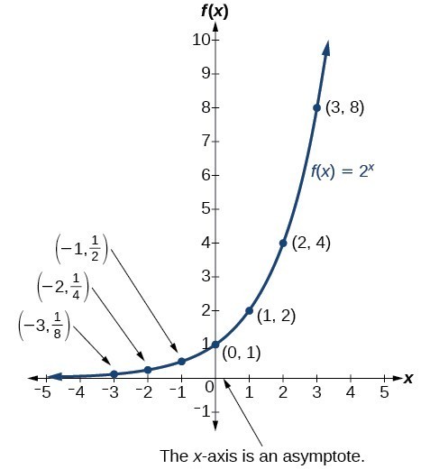
In the graph, notice that the graph gets close to the x-axis, but never touches it.

The feature that the graph is always positive, yet gets closer and closer to the [latex]x[/latex]-axis as [latex]x[/latex] gets smaller (heading toward negative infinity) is a new idea for us. Such a line that the graph approaches in the long run is called an asymptote. So for this function, the [latex]x[/latex]-axis (i.e. the line [latex]y=0[/latex]) is an asymptote; more specifically, it is a horizontal asymptote.

The domain of [latex]f\left(x\right)={2}^{x}[/latex] is all real numbers; the range is [latex]\left(0,\infty \right)[/latex].

Below is a video demonstration of graphing the same function we graphed above.

Let us consider another example, this time with a fractional base. Let [latex]g(x)=\left(\frac{1}{2}\right)^{x}[/latex]. We arrive at the following set of points.

Notice from the table that:

• the output values are positive for all values of x;
• as x increases, the output values grow smaller, approaching zero; and
• as x decreases, the output values grow without bound.

The graph shows the exponential decay function, [latex]g\left(x\right)={\left(\frac{1}{2}\right)}^{x}[/latex].

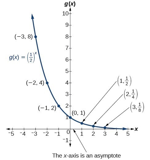
The domain of [latex]g\left(x\right)={\left(\frac{1}{2}\right)}^{x}[/latex] is all real numbers; the range is [latex]\left(0,\infty \right)[/latex]. Also similar to our previous example, the [latex]x[/latex]-axis is a horizontal asymptote, although this time, the graph approaches this line as [latex]x[/latex] increases to positive infinity.

While there are obviously infinitely more bases we could examine, these two examples tell us a tremendous amount about exponential functions, which we summarize below.

Characteristics of the Graph of  [latex]f(x) = a^{x}[/latex]

An exponential function of the form [latex]f\left(x\right)={a}^{x}[/latex], [latex]a>0[/latex], [latex]a\ne 1[/latex], has these characteristics:

• domain: [latex]\left(-\infty , \infty \right)[/latex]
• range: [latex]\left(0,\infty \right)[/latex]
• x-intercept: none
• y-intercept: [latex]\left(0,1\right)[/latex]
• increasing if [latex]a>1[/latex], called exponential growth
• decreasing if [latex]0<a<1[/latex], called exponential decay

Compare the general graphs of exponential growth and decay functions below.

In our first example, we will plot an exponential growth function where the base is 3. This will help confirm our claim above that, while the individual points will vary, the overall shape will correspond to those shown above.

So far, we have only considered basic exponential functions of the form [latex]f(x)=a^x[/latex]. In the next example, we return to a base of 2, but this time we will introduce an additional number in the exponent as we graph [latex]f(x)=2^{x-3}[/latex]. While we will still create a table to aid us in our graph, if we were to select the same set of values that we have chosen in all previous examples, we would not yet see the traditional shape we have come to expect. To rectify this, we instead choose [latex]x[/latex]-values around [latex]x=3[/latex]. The reason for this choice is that this is the [latex]x[/latex]-value that will result in an exponent of zero. One way of thinking about this is that the point [latex](0,1)[/latex] that we have encountered in every graph is now being shifted over to [latex](3,1)[/latex] instead.

Example 2

Sketch a graph of [latex]f(x)={2}^{x-3}[/latex].

Show Solution

Before graphing, identify the behavior and create a table of points for the graph.

• Since [latex]a=2[/latex], which is greater than one, we know the function is increasing (exponential growth), and we can verify this by creating a table of values. The left tail of the graph will get really close to the x-axis and the right tail will increase without bound.
• Create a table of points, but now selecting values around [latex]x=3[/latex].
  

  x	[latex]1[/latex]	[latex]2[/latex]	[latex]3[/latex]	[latex]4[/latex]	[latex]5[/latex]
  [latex]f\left(x\right)=2^{x-3}[/latex]	[latex]\frac{1}{4}[/latex]	[latex]\frac{1}{2}[/latex]	[latex]1[/latex]	[latex]2[/latex]	[latex]4[/latex]

This leads to the following graph:

What we want to observe about the graph in the last example is that the overall shape and many of the graphical features were preserved, but the whole graph was moved to the right by 3 units.

In our last example, we revisit bases smaller than 1, but again with an additional number in the exponent.

Example 3

Sketch a graph of [latex]f(x)=\left(\frac{1}{4}\right)^{x+2}[/latex].

Show Solution

Before graphing, identify the behavior and create a table of points for the graph.

• Since [latex]a=\frac{1}{4}[/latex], which is less than one, we know the function is decreasing (exponential decay). The right tail of the graph will get really close to the x-axis and the left tail will increase without bound.
• Create a table of points, but now selecting values around [latex]x=-2[/latex] as this is the value that would result in a zero exponent.
  

  x	[latex]-4[/latex]	[latex]-3[/latex]	[latex]-2[/latex]	[latex]-1[/latex]	[latex]0[/latex]
  [latex]f\left(x\right)=\left(\frac{1}{4}\right)^{x+2}[/latex]	[latex]16[/latex]	[latex]4[/latex]	[latex]1[/latex]	[latex]\frac{1}{4}[/latex]	[latex]\frac{1}{16}[/latex]

This results in the following graph:

If you would like to explore a little different situation, watch the video below. Here, you will see the effect of a constant multiplier in front of the exponential.

The Natural Number e

While most people have heard of the number [latex]\pi[/latex], there is another constant in mathematics that appears in numerous calculations, but sadly does not receive nearly the same attention outside of STEM courses. This is the natural number e. Similar to [latex]\pi[/latex], the natural number is irrational and has an approximate value of [latex]e\approx 2.718281828[/latex]. The natural number appears in situations ranging from population growth, radioactive decay, and continuously compounded interest to the spirals we see in shells and entire spiral galaxies.

To find a power of e, we will want to use a scientific calculator. The button varies by model of calculator, but often looks like [latex]e^{x}[/latex]. It may require using a 2nd function or shift feature as well. In addition, on some calculators, you might push the “e” button and then the desired power, whereas on others this may be reversed. To try this out on your calculator, try computing [latex]e^{2}[/latex]. You should get

[latex]e^2\approx 7.389[/latex]

While e has many special mathematical properties, on the other hand, it is still some number larger than 1. As such, we already know what the basic shape of the function [latex]f(x)=e^x[/latex] will look like graphically, exhibiting exponential growth. We proceed by making an [latex]xy[/latex]-table. Try using your calculator to verify the values given below (rounded to the nearest thousandth).

Plotting these points yields the following graph:

As expected, we see similarities to our earlier examples, with a y-intercept at (0,1) and the x-axis serving as a horizontal asymptote.

Summary

Graphs of exponential growth functions will have a right tail that increases without bound and a left tail that gets really close to the x-axis, making the x-axis an asymptote. On the other hand, graphs of exponential decay functions will have a left tail that increases without bound and a right tail that gets really close to the x-axis. Points can be generated with a table of values which can then be used to graph the function.