Section 8.3 Learning Objectives
8.3: Graphing Absolute Value and Quadratic Functions
- Graph basic absolute value functions
- Graph basic quadratic functions
The Basic Absolute Value Function
In Chapter 2, we reviewed the idea of absolute value and introduced strategies to solve absolute value equations and inequalities. In this section, our goal is to graph absolute value functions.
Let us begin with the most basic absolute value function, [latex]f(x)=|x|.[/latex]
Recall that the absolute value of a number is its distance from zero on the number line. As with any function, we can use a table to assist us in graphing it.
Since we are unsure of the shape, we want to pick several points, including positives and negatives. This leads to the table given below.
| [latex]x[/latex] | [latex]f(x)=|x|[/latex] |
| [latex]-3[/latex] | [latex]|-3|=3[/latex] |
| [latex]-2[/latex] | [latex]|-2|=2[/latex] |
| [latex]-1[/latex] | [latex]|-1|=1[/latex] |
| [latex]0[/latex] | [latex]|0|=0[/latex] |
| [latex]1[/latex] | [latex]|1|=1[/latex] |
| [latex]2[/latex] | [latex]|2|=2[/latex] |
| [latex]3[/latex] | [latex]|3|=3[/latex] |
Next we plot the points.

Had we not chosen enough points, we may be tempted to draw something more like a smooth curve through the points. However, we can see that this will require a graph that is more linear, except that it seems to suddenly change directions at the origin. Had we only chosen points to the right of 0, we may have thought the graph would be a simple straight line instead of the “V” shape that is ends up being. The final graph of [latex]f(x)=|x|[/latex] is shown below.

This “V” shape will appear in all of the simple absolute value functions we will consider in this section. However, the “V” might be shifted, made narrower or wider, or even flipped.
Graphing Absolute Value Functions of the Form [latex]f(x)=a|x|+b[/latex]
Knowing the basic shape of an absolute value graph will help us as we continue our exploration of absolute values.
Consider the function [latex]f(x)=|x|-3[/latex]. Let us try plugging in the same values for [latex]x[/latex] that we use for the basic absolute value function.
| [latex]x[/latex] | [latex]f(x)=|x|-3[/latex] |
| [latex]-3[/latex] | [latex]|-3|-3=3-3=0[/latex] |
| [latex]-2[/latex] | [latex]|-2|-3=2-3=-1[/latex] |
| [latex]-1[/latex] | [latex]|-1|-3=1-3=-2[/latex] |
| [latex]0[/latex] | [latex]|0|-3=0-3=-3[/latex] |
| [latex]1[/latex] | [latex]|1|-3=1-3=-2[/latex] |
| [latex]2[/latex] | [latex]|2|-3=2-3=-1[/latex] |
| [latex]3[/latex] | [latex]|3|-3=3-3=0[/latex] |
Plotting these points gives the graph shown below.

We see that same “V” shape, which we will come to expect with this type of absolute value function. However, not coincidentally, notice that the curve has moved down 3 units.
Example 1
Graph [latex]f(x)=|x|+2[/latex].

Strategy for Graphing Absolute Value Functions of the Form [latex]f(x)=a|x|+b[/latex]
- Make an [latex]xy[/latex]-table. We recommend (at least) five values for [latex]x[/latex], [latex]x=-2,-1,0,1,2[/latex].
- Graph. The resulting curve should have a “V” shape.
In the next problem, we will see what happens when there is a coefficient other than 1 in front of the absolute value.
Example 2
Graph [latex]f(x)=2|x|[/latex].

In our last example, we combine some of the ideas we have seen. Moreover, we look at the effect of a negative coefficient.
Example 3
Graph [latex]f(x)=-2|x|+1[/latex].

If you would like to investigate further into absolute value graphs, check out the “Think About It” below.
think about it
Graph [latex]f(x)=|x-3|[/latex].

Graphing Basic Quadratic Functions
In Modules 5 and 6 we learned about polynomials. An equation containing a second-degree polynomial is called a quadratic equation. For example, equations such as [latex]{x}^{2}-3x-4=0[/latex] and [latex]{x}^{2}-16=0[/latex] are in the “family” of quadratic equations. They are used in countless ways in the fields of engineering, architecture, finance, biological science, and, of course, mathematics.
Just like the functions in other “families” we’ve learned about (linear, exponential, absolute value), quadratic functions can also be graphed. It is helpful to have an idea about what the shape should be so you can be sure that you have chosen enough points to plot as a guide. Let us start with the most basic quadratic function, [latex]f(x)=x^{2}[/latex].
Graph [latex]f(x)=x^{2}[/latex].
We’ll start with a table of values. Then think of each row of the table as an ordered pair.
| [latex]x[/latex] | [latex]f(x)=x^2[/latex] |
| [latex]−2[/latex] | [latex](-2)^2=4[/latex] |
| [latex]−1[/latex] | [latex](-1)^2=1[/latex] |
| [latex]0[/latex] | [latex](0)^2=0[/latex] |
| [latex]1[/latex] | [latex](1)^2=1[/latex] |
| [latex]2[/latex] | [latex](2)^2=4[/latex] |
Now we’ll plot the points [latex](-2,4), (-1,1), (0,0), (1,1), (2,4)[/latex]
At first glance, it might appear that these points make a “V” shape like the absolute value functions we have graphed previously. But, the quadratic family of functions is not drawn using straight lines. Since the points are not on a line, you cannot use a straight edge. Connect the points as best you can using a smooth curve (not a series of straight lines). You may want to find and plot additional points (such as the ones in blue below). Placing arrows on the tips of the lines implies that they continue in that direction forever.
Notice that the shape is similar to the letter U. This is called a parabola. One-half of the parabola is a mirror image of the other half. The lowest point on this graph is called the vertex. The vertical line that goes through the vertex is called the line of symmetry. In this case, that line is the y-axis, which is the line [latex]x=0[/latex].
In the following video, we show an example of graphing another quadratic function, [latex]f(x)=\frac{1}{2}x^2[/latex], using a table of values.
The equations for quadratic functions can be written in the form [latex]f(x)=ax^{2}+bx+c[/latex] (where [latex]a\ne 0[/latex]). In the two basic quadratic functions we graphed above, notice there was only the [latex]ax^2[/latex] term and that both [latex]b=0[/latex], and [latex]c=0[/latex] for those functions.
Although there are many forms that quadratic functions can be written in, this Elementary Algebra course will focus only on graphing basic quadratic functions of the form [latex]f(x)=ax^{2}+c[/latex].
Quadratic functions of the form [latex]f(x)=ax^{2}+c[/latex] will always be centered around the y-axis which is the line [latex]x=0[/latex].
We have shared two examples above of graphing a basic quadratic function of the form [latex]f(x)=ax^{2}+c[/latex], where [latex]c=0[/latex], so let’s now explore how to graph a quadratic function of the form [latex]f(x)=ax^{2}+c[/latex] where [latex]c\ne 0[/latex] .
Graph [latex]f(x)=x^{2}-4[/latex].
Similar to the problems above, lets start with a table of values.
| [latex]x[/latex] | [latex]f(x)=x^2-4[/latex] | [latex]f(x)[/latex] |
| [latex]−2[/latex] | [latex](-2)^2-4 = 4-4 = 0[/latex] | 0 |
| [latex]−1[/latex] | [latex](-1)^2-4 = 1-4 = -3[/latex] | -3 |
| [latex]0[/latex] | [latex](0)^2-4 = 0-4 = -4[/latex] | -4 |
| [latex]1[/latex] | [latex](1)^2-4 = 1-4 = -3[/latex] | -3 |
| [latex]2[/latex] | [latex](2)^2-4 = 4-4 = 0[/latex] | 0 |
We’ll now plot the points [latex](-2,0), (-1,-3), (0,-4), (1,-3), (2,0)[/latex] on the graph.

If we connect all the points with a smooth curve we will have the graph of our function [latex]f(x)=x^{2}-4[/latex].

Let’s have you now try one on your own:
Example 4
Graph the function: [latex]f(x)=x^2-16[/latex]


Lets try a few more examples.
Example 5
Graph the function: [latex]f(x)=x^2+5[/latex]

In the next example we will explore how parabolas don’t always open upwards.
Example 6
Graph the function: [latex]f(x)=-3x^2[/latex]


As we saw with the last example, with quadratic functions of the form [latex]f(x)=ax^{2}+c[/latex], changing the value of [latex]a[/latex] can change the width of the parabola and whether it opens up ([latex]a>0[/latex]) or down ([latex]a<0[/latex]). If [latex]a[/latex] is positive, the vertex is the lowest point, and the parabola opens up. If [latex]a[/latex] is negative, the vertex is the highest point, and the parabola opens down.
When graphing quadratic functions of the form [latex]f(x)=ax^{2}+c[/latex] follow the steps below:
- Recognize the form of the quadratic function and that it will be a parabola centered around x=0.
- Make a table of values, making sure to choose some values on either side of x=0, as well as the value of x=0
- Plot your points and connect them with a smooth curve into a parabola shape.
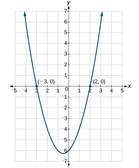
Think About it
Graph the equation: [latex]f(x)={x}^{2}+x - 6[/latex]. (It may be helpful to factor it, and set it equal to 0 to find the [latex]x[/latex]-intercepts.)
Graphing Quadratics Summary
Creating a graph of a function is one way to understand the relationship between the inputs and outputs of that function. Creating a graph can be done by choosing values for x, finding the corresponding y values, and plotting them. However, it helps to understand the basic shape of the function. Knowing how changes to the basic function equation affect the graph is also helpful.
The shape of a quadratic function is a parabola. Parabolas have the equation [latex]f(x)=ax^{2}+bx+c[/latex], where [latex]a, b[/latex] and [latex]c[/latex] are real numbers and [latex]a\ne0[/latex]. The value of [latex]a[/latex] determines the width and the direction of the parabola, while the vertex depends on the values of [latex]a, b[/latex] and [latex]c[/latex].
Candela Citations
- Authored by: James Sousa (Mathispower4u.com) . Located at: https://www.youtube.com/watch?v=X_gqB9bVOVE&feature=youtu.be%2F. License: CC BY: Attribution