Recognizing Characteristics of Graphs of Polynomial Functions

Polynomial functions of degree 2 or more have graphs that do not have sharp corners. These types of graphs are called smooth curves. Polynomial functions also display graphs that have no breaks. Curves with no breaks are called continuous. Figure 1 shows a graph that represents a polynomial function on the left and a graph that represents a function that is not a polynomial on the right.

Figure 1

Example 1:  Recognizing Polynomial Functions

Which of the graphs in Figure 2 and Figure 3 represent a polynomial function?

Figure 2

Figure 3

Show Solution

The graphs of [latex]f[/latex] and [latex]h[/latex] are graphs of polynomial functions. They are smooth and continuous.

The graphs of [latex]g[/latex] and [latex]k[/latex] are graphs of functions that are not polynomials. The graph of function [latex]g[/latex] has a sharp corner. The graph of function [latex]k[/latex] is not continuous.

Using Factoring to Find Zeros of Polynomial Functions

Recall that if [latex]f[/latex] is a polynomial function, the values of [latex]x[/latex] for which [latex]f\left(x\right)=0[/latex] are called zeros of [latex]f.[/latex] If the equation of the polynomial function can be factored, we can set each factor equal to zero and solve for the zeros.

We can use this method to find [latex]x\text{-}[/latex]intercepts because at the [latex]x\text{-}[/latex]intercepts, we find the input values when the output value is zero. For general polynomials, this can be a challenging prospect. While quadratics can be solved using the relatively simple quadratic formula, the corresponding formulas for cubic and fourth-degree polynomials are not simple enough to remember, and formulas do not exist for general higher-degree polynomials. Consequently, we will limit ourselves to three cases in this section:

1. The polynomial can be factored using known methods: greatest common factor and trinomial factoring.
2. The polynomial is given in factored form.
3. Technology is used to determine the intercepts.[latex]\\[/latex]

Example 2:  Finding the x-Intercepts of a Polynomial Function by Factoring

Find the x-intercepts of [latex]f\left(x\right)={x}^{6}-3{x}^{4}+2{x}^{2}.[/latex]

Show Solution

We can attempt to factor this polynomial to find solutions for [latex]f\left(x\right)=0.[/latex]

[latex]\begin{align*}{x}^{6}-3{x}^{4}+2{x}^{2}&=0&&\text{ }\\\text{ }{x}^{2}\left({x}^{4}-3{x}^{2}+2\right)&=0\hfill && \text{Factor out the greatest common factor}.\hfill \\ {x}^{2}\left({x}^{2}-1\right)\left({x}^{2}-2\right)&=0\hfill && \text{Factor the trinomial}.\hfill \end{align*}[/latex]

[latex]\\[/latex]

Set each factor equal to zero.

[latex]x^2=0\text{ }\text{ }\text{ }\text{ or }\text{ }\text{ }\text{ }\left({x}^{2}-1\right)=0\text{ }\text{ }\text{ }\text{ or }\text{ }\text{ }\text{ }\left({x}^{2}-2\right)=0[/latex][latex]\\[/latex]

Solving each of these equations gives

[latex]\begin{array}{lllllllll}\\ {x}^{2}=0\hfill & \hfill & \text{or}\hfill & \hfill & \text{ }{x}^{2}=1\hfill & \hfill & \text{or}\hfill & \hfill & \text{ }\text{ }{x}^{2}=2\hfill \\ \text{ }x=0\hfill & \hfill & \hfill & \hfill & \text{ }x=±1\hfill & \hfill & \hfill & \hfill & \text{ }\text{ }x=±\sqrt[\leftroot{1}\uproot{2} ]{2}.\hfill \end{array}[/latex]

[latex]\\[/latex]

This gives us five [latex]x\text{-}[/latex]intercepts: [latex]\left(0,0\right),\left(1,0\right),\left(-1,0\right),\left(\sqrt[\leftroot{1}\uproot{2} ]{2},0\right),[/latex] and [latex]\left(-\sqrt[\leftroot{1}\uproot{2} ]{2},0\right).[/latex] See Figure 4. We can see that this is an even function.

Figure 4

Example 3:  Finding the x-Intercepts of a Polynomial Function by Factoring

Find the [latex]x\text{-}[/latex]intercepts of [latex]f\left(x\right)={x}^{3}-5{x}^{2}-x+5.[/latex]

Show Solution

Find solutions for [latex]f\left(x\right)=0[/latex] by factoring.

[latex]\begin{align*}\text{ }{x}^{3}-5{x}^{2}-x+5&=0&&\text{ } \\ \text{ }{x}^{2}\left(x-5\right)-\left(x-5\right)&=0\hfill && \text{Factor by grouping}.\hfill \\ \text{ }\left({x}^{2}-1\right)\left(x-5\right)&=0\hfill && \text{Factor out the common factor}.\hfill \\ \left(x+1\right)\left(x-1\right)\left(x-5\right)&=0\hfill && \text{Factor the difference of squares}.\hfill \end{align*}[/latex]

[latex]\\[/latex]

Set each factor equal to zero and solve.

[latex]\begin{array}{lllll}x+1=0\hfill & \text{or}\hfill & x-1=0\hfill & \text{or}\hfill & x-5=0\hfill \\ \text{ }\text{ }\text{ }\text{ }\text{ }\text{ }\text{ }\text{ }x=-1\hfill & \hfill & \text{ }\text{ }\text{ }\text{ }\text{ }\text{ }\text{ }\text{ }x=1\hfill & \hfill & \text{ }\text{ }\text{ }\text{ }\text{ }\text{ }\text{ }\text{ }\text{ }x=5\hfill \end{array}[/latex]

 [latex]\\[/latex]

There are three [latex]x\text{-}[/latex]intercepts: [latex]\left(-1,0\right),\left(1,0\right),[/latex] and [latex]\left(5,0\right).[/latex] See Figure 5.

Figure 5

Example 4:  Finding the y– and x-Intercepts of a Polynomial in Factored Form

Find the [latex]y\text{-}[/latex] and x-intercepts of [latex]g\left(x\right)={\left(x-2\right)}^{2}\left(2x+3\right).[/latex]

Show Solution

The y-intercept can be found by evaluating [latex]g\left(0\right).[/latex]

[latex]\begin{align*}g\left(0\right)&={\left(0-2\right)}^{2}\left(2\left(0\right)+3\right)\\ &=12\end{align*}[/latex]

[latex]\\[/latex]

So the y-intercept is [latex]\left(0,12\right).[/latex]

The x-intercepts can be found by solving [latex]g\left(x\right)=0.[/latex]

[latex]{\left(x-2\right)}^{2}\left(2x+3\right)=0[/latex]

[latex]\\[/latex]

[latex]\begin{array}{lllll}{\left(x-2\right)}^{2}=0\hfill & \hfill & \text{or}\hfill & \hfill & \left(2x+3\right)=0\hfill \\ \text{ }x-2=0\hfill & \hfill & \hfill & \hfill & \text{ }x=-\frac{3}{2}\hfill \\ \text{ }x=2\hfill & \hfill & \hfill & \hfill & \hfill \end{array}[/latex]

[latex]\\[/latex]

So the [latex]x\text{-}[/latex]intercepts are [latex]\left(2,0\right)[/latex] and [latex]\left(-\frac{3}{2},0\right).[/latex]

Analysis

We can always check that our answers are reasonable by using a graphing calculator to graph the polynomial as shown in Figure 6.

Figure 6

Example 5:  Finding the x-Intercepts of a Polynomial Function Using a Graph

Find the [latex]x\text{-}[/latex]intercepts of [latex]h\left(x\right)={x}^{3}+4{x}^{2}+x-6.[/latex]

The graph of this function, is in Figure 7.

Figure 7

Show Solution

This polynomial is not in factored form, has no common factors, and does not appear to be factorable using techniques previously discussed. Fortunately, we can use technology to find the intercepts. Keep in mind that some values make graphing difficult by hand. In these cases, we can take advantage of graphing utilities.

Looking at the graph of this function, as shown in Figure 7, it appears that there are x-intercepts at [latex]x=-3,-2,[/latex] and [latex]1.[/latex]

We can check whether these are correct by substituting these values for [latex]x[/latex] and verifying that

[latex]h\left(-3\right)=h\left(-2\right)=h\left(1\right)=0.[/latex]

[latex]\\[/latex]

Since [latex]h\left(x\right)={x}^{3}+4{x}^{2}+x-6,[/latex] we have:

[latex]\begin{align*}h\left(-3\right)&={\left(-3\right)}^{3}+4{\left(-3\right)}^{2}+\left(-3\right)-6=-27+36-3-6=0\\ h\left(-2\right)&={\left(-2\right)}^{3}+4{\left(-2\right)}^{2}+\left(-2\right)-6=-8+16-2-6=0\\ h\left(1\right)&={\left(1\right)}^{3}+4{\left(1\right)}^{2}+\left(1\right)-6=1+4+1-6=0\end{align*}[/latex]

[latex]\\[/latex]

Each [latex]x\text{-}[/latex]intercept corresponds to a zero of the polynomial function and each zero yields a factor, so we can now write the polynomial in factored form.

[latex]\begin{align*}h\left(x\right)&={x}^{3}+4{x}^{2}+x-6\hfill \\ \text{ }&=\left(x+3\right)\left(x+2\right)\left(x-1\right)\hfill \end{align*}[/latex]

Identifying Zeros and Their Multiplicities

Graphs behave differently at various [latex]x\text{-}[/latex]intercepts. Sometimes, the graph will cross over the horizontal axis at an intercept. Other times, the graph will touch the horizontal axis and bounce off.

Suppose, for example, we graph the function  [latex]f\left(x\right)=\left(x+3\right){\left(x-2\right)}^{2}{\left(x+1\right)}^{3}.[/latex]

Notice in Figure 8 that the behavior of the function at each of the [latex]x\text{-}[/latex]intercepts is different.

Figure 8 Identifying the behavior of the graph at an x-intercept by examining the multiplicity of the zero.

The [latex]x\text{-}[/latex]intercept [latex]-3[/latex] is the solution of equation [latex]\left(x+3\right)=0.[/latex] The graph passes directly through the [latex]x\text{-}[/latex]intercept at [latex]x=-3.[/latex] The factor is linear (has a degree of 1), so the behavior near the intercept is like that of a line—it passes directly through the intercept. We call this a single zero because the zero corresponds to a single factor of the function.

The [latex]x\text{-}[/latex]intercept at [latex]x=2[/latex] is the repeated solution of equation [latex]{\left(x-2\right)}^{2}=0.[/latex] The graph touches the axis at the intercept and changes direction. The factor is quadratic (degree 2), so the behavior near the intercept is like that of a quadratic—it bounces off of the horizontal axis at the [latex]x\text{-}[/latex]intercept.

The factor is repeated, that is, the factor [latex]\left(x-2\right)[/latex] appears twice. The number of times a given factor appears in the factored form of the equation of a polynomial is called the multiplicity. The zero associated with this factor, [latex]x=2,[/latex] has multiplicity 2 because the factor [latex]\left(x-2\right)[/latex] occurs twice.

The [latex]x\text{-}[/latex]intercept at [latex]x=-1[/latex] is the repeated solution of factor [latex]{\left(x+1\right)}^{3}=0.[/latex] The graph passes through the axis at the intercept, but flattens out a bit first. This factor is cubic (degree 3), so the behavior near the intercept is like that of a cubic—with the same S-shape near the intercept as the toolkit function [latex]f\left(x\right)={x}^{3}.[/latex] We call this a triple zero, or a zero with multiplicity 3.

For zeros with even multiplicities, the graphs touch or are tangent to the [latex]x\text{-}[/latex]axis. For zeros with odd multiplicities, the graphs cross or intersect the [latex]x\text{-}[/latex]axis. See Figure 9 for examples of graphs of polynomial functions with multiplicity 1, 2, and 3.

Figure 9

For higher even powers, such as 4, 6, and 8, the graph will still touch and bounce off of the horizontal axis but, for each increasing even power, the graph will appear flatter as it approaches and leaves the [latex]x\text{-}[/latex]axis.

For higher odd powers, such as 5, 7, and 9, the graph will still cross through the horizontal axis, but for each increasing odd power, the graph will appear flatter as it approaches and leaves the [latex]x\text{-}[/latex]axis.

Example 6:  Identifying Zeros and Their Multiplicities

Use the graph of the function of degree 6 in Figure 10 to identify the zeros of the function and their possible multiplicities.

Figure 10

Show Solution

The polynomial function is of degree [latex]6.[/latex] The sum of the multiplicities must be [latex]6.[/latex]

Starting from the left, the first zero occurs at [latex]x=-3.[/latex] The graph touches the x-axis, so the multiplicity of the zero must be even. The zero of [latex]-3[/latex] could have multiplicity [latex]2.[/latex]

The next zero occurs at [latex]x=-1.[/latex] The graph looks almost linear at this point. This is a single zero of multiplicity 1.

The last zero occurs at [latex]x=4.[/latex] The graph crosses the x-axis, so the multiplicity of the zero must be odd. We know that the multiplicity is 3 so that the sum of the multiplicities is 6.

Try it #2

Use the graph of the function of degree 9 in Figure 11 to identify the zeros of the function and their multiplicities.

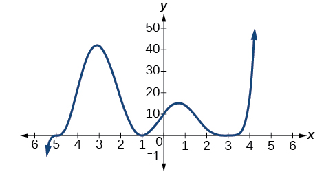
Figure 11

Show Solution

The graph has a zero at [latex]x= -5[/latex] with multiplicity 3, a zero at [latex]x=-1[/latex] with multiplicity 2, and a zero at [latex]x=3[/latex] with multiplicity 4.

Determining End Behavior

As we have already learned, the behavior of a graph of a polynomial function of the form

will either ultimately rise or fall as [latex]x[/latex] increases without bound and will either rise or fall as [latex]x[/latex] decreases without bound. This is because for very large inputs, say 100 or 1,000, the leading term dominates the size of the output. The same is true for more and more negative inputs, say –100 or –1,000.

Recall that we call this behavior the end behavior of a function. When the leading term of a polynomial function, [latex]{a}_{n}{x}^{n},[/latex] is an even power function with a positive leading coefficient, as [latex]x[/latex] increases or decreases without bound, [latex]f\left(x\right)[/latex] increases without bound. When the leading term is an odd power function with a positive leading coefficient, as [latex]x[/latex] decreases without bound, [latex]f\left(x\right)[/latex] also decreases without bound; as [latex]x[/latex] increases without bound, [latex]f\left(x\right)[/latex] also increases without bound. If the leading coefficient is negative, it will change the direction of the end behavior. Figure 12 summarizes all four cases.

Figure 12

Understanding the Relationship between Degree and Turning Points

In addition to the end behavior, recall that we can analyze a polynomial function’s local behavior. It may have a turning point where the graph changes from increasing to decreasing (rising to falling or a local maximum) or decreasing to increasing (falling to rising or a local minimum). Look at the graph of the polynomial function [latex]f\left(x\right)={x}^{4}-{x}^{3}-4{x}^{2}+4x[/latex] in Figure 13. The graph has three turning points.

This function [latex]f[/latex] is a 4^th degree polynomial function and has 3 turning points. The maximum number of turning points of a polynomial function is always one less than the degree of the function.

Graphing Polynomial Functions

We can use what we have learned about multiplicities, end behavior, and turning points to sketch graphs of polynomial functions. Let us put this all together and look at the steps required to graph polynomial functions.

Example 8:  Sketching the Graph of a Polynomial Function

Sketch a graph of [latex]f\left(x\right)=-2{\left(x+3\right)}^{2}\left(x-5\right).[/latex]

Show Solution

This graph has two [latex]x\text{-}[/latex]intercepts. At [latex]x=-3,[/latex] the factor is squared, indicating a multiplicity of 2. The graph will bounce at this [latex]x\text{-}[/latex]intercept. At [latex]x=5,[/latex] the function has a multiplicity of one, indicating the graph will cross through the axis at this intercept.

The y-intercept is found by evaluating [latex]f\left(0\right).[/latex]

[latex]\begin{align*}f\left(0\right)&=-2{\left(0+3\right)}^{2}\left(0-5\right)\hfill \\ \text{ }&=-2\cdot 9\cdot \left(-5\right)\hfill \\ \text{ }&=90\hfill \end{align*}[/latex]

[latex]\\[/latex]

The [latex]y\text{-}[/latex]intercept is [latex]\left(0,90\right).[/latex]

Additionally, we can see the leading term, if this polynomial were multiplied out, would be [latex]-2{x}^{3},[/latex] so the end behavior is that of a vertically reflected cubic, with the outputs decreasing as the inputs increase without bound, and the outputs increasing as the inputs decrease without bound. See Figure 14.

Figure 14

To sketch this, we consider that:

• As [latex]x\to -\infty [/latex] the function [latex]f\left(x\right)\to \infty ,[/latex] so we know the graph starts in the second quadrant and is decreasing toward the [latex]x\text{-}[/latex]axis.
• Since [latex]f\left(-x\right)=-2{\left(-x+3\right)}^{2}\left(-x–5\right)[/latex] is not equal to [latex]f\left(x\right),[/latex] the graph does not display symmetry.
• At [latex]\left(-3,0\right),[/latex] the graph bounces off of the [latex]x\text{-}[/latex]axis, so the function must start increasing.

  At [latex]\left(0,90\right),[/latex] the graph crosses the [latex]y\text{-}[/latex]axis at the [latex]y\text{-}[/latex]intercept. See Figure 15.

Figure 15

Somewhere after this point, the graph must turn back down or start decreasing toward the horizontal axis because the graph passes through the next intercept at [latex]\left(5,0\right).[/latex] See Figure 16.

Figure 16

As [latex]x\to \infty [/latex] the function [latex]f\left(x\right)\to \mathrm{-\infty },[/latex] so we know the graph continues to decrease, and we can stop drawing the graph in the fourth quadrant.

Using technology, we can create the graph for the polynomial function, shown in Figure 17, and verify that the resulting graph looks like our sketch in Figure 16.

Figure 17  The complete graph of the polynomial function [latex]f\left(x\right)=-2{\left(x+3\right)}^{2}\left(x-5\right).[/latex]

Try it #3

Sketch a graph of [latex]f\left(x\right)=\frac{1}{4}x{\left(x-1\right)}^{4}{\left(x+3\right)}^{3}.[/latex]

Show Solution