Local Behavior of [latex]f\left(x\right)=\frac{1}{x}[/latex]

Let’s begin by looking at the reciprocal function, [latex]f\left(x\right)=\frac{1}{x}.[/latex] We cannot divide by zero, which means the function is undefined at [latex]x=0;[/latex] so zero is not in the domain. As the input values approach zero from the left side (negative values very close to zero), the function values decrease without bound. We can see this behavior in Table 2.

We write in arrow notation, as [latex]x\to {0}^{-},f\left(x\right)\to -\infty [/latex].

As the input values approach zero from the right side (positive values very close to zero), the function values increase without bound. We can see this behavior in Table 3.

We write in arrow notation as [latex]x\to {0}^{+}, f\left(x\right)\to \infty .[/latex]

See Figure 2.

Figure 2

This behavior creates a vertical asymptote, which is a vertical line that the graph approaches but never crosses. In this case, the graph is approaching the vertical line [latex]x=0[/latex] as the input becomes close to zero. See Figure 3.

Figure 3

End Behavior of [latex]f\left(x\right)=\frac{1}{x}[/latex]

As the values of [latex]x[/latex] increase without bound, the function values approach 0. As the values of [latex]x[/latex] decrease without bound, the function values approach 0. See Figure 4. Symbolically, using arrow notation

[latex]\textrm{as }x\to \infty ,f\left(x\right)\to 0,\textrm{and as }x\to -\infty ,f\left(x\right)\to 0.[/latex]

Figure 4

Based on this overall behavior and the graph, we can see that the function approaches 0 but never actually reaches 0; it seems to level off as the inputs become large. This behavior creates a horizontal asymptote, a horizontal line that the graph approaches as the input increases or decreases without bound. In this case, the graph is approaching the horizontal line [latex]y=0.[/latex] See Figure 5.

Figure 5

Example 1:  Using Arrow Notation

Use arrow notation to describe the end behavior and local behavior of the function graphed in Figure 6.

Figure 6

Show Solution

Notice that the graph is showing a vertical asymptote at [latex]x=2,[/latex] which tells us that the function is undefined at [latex]x=2.[/latex]

As [latex]x\to {2}^{-},f\left(x\right)\to -\infty ,[/latex] and as [latex]x\to {2}^{+},\text{ }f\left(x\right)\to \infty .[/latex]

Also, as the inputs decrease without bound, the graph appears to be leveling off with output values closer and closer to 4, indicating a horizontal asymptote at [latex]y=4.[/latex] As the inputs increase without bound, the graph levels off approaching 4.

As [latex]x\to \infty ,\text{ }f\left(x\right)\to 4[/latex] and as [latex]x\to -\infty ,\text{ }f\left(x\right)\to 4.[/latex]

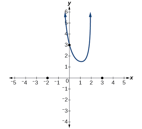
Example 2:  Using Transformations to Graph a Rational Function

Sketch a graph of the reciprocal function shifted two units to the left and up three units. Identify the horizontal and vertical asymptotes of the graph, if any.

Show Solution

Shifting the graph left 2 and up 3 would result in the function

[latex]f\left(x\right)=\frac{1}{x+2}+3,[/latex]

[latex]\\[/latex]

or equivalently, by adding the terms after finding a common denominator,

[latex]f\left(x\right)=\frac{3x+7}{x+2}.[/latex]

[latex]\\[/latex]

The graph of the shifted function is displayed in Figure 7.

Figure 7

Notice that this function is undefined at [latex]x=-2,[/latex] and the graph also is showing a vertical asymptote at [latex]x=-2.[/latex]

As [latex]x\to -{2}^{-}, f\left(x\right)\to -\infty ,[/latex] and as [latex]x\to -{2}^{+}, f\left(x\right)\to \infty .[/latex]

[latex]\\[/latex]

As the inputs increase and decrease without bound, the graph appears to be leveling off with output values getting closer and closer to 3, indicating a horizontal asymptote of [latex]y=3.[/latex]

As [latex]x\to ±\infty , f\left(x\right)\to 3.[/latex]

Analysis

Notice that horizontal and vertical asymptotes are shifted left 2 and up 3 along with the function.

Try it #2

Sketch the graph, and find the horizontal and vertical asymptotes of the reciprocal squared function that has been shifted right 3 units and down 4 units.

Show Solution

Figure 8

The function and the asymptotes are shifted 3 units right and 4 units down. As [latex]x\to 3,f\left(x\right)\to \infty ,[/latex] and as [latex]x\to ±\infty ,f\left(x\right)\to -4.[/latex] Therefore, the vertical asymptote is  [latex]x=3,[/latex] and the horizontal asymptote is  [latex]y=-4.[/latex]

The function is [latex]f\left(x\right)=\frac{1}{{\left(x-3\right)}^{2}}-4.[/latex]

Finding the Domains of Rational Functions

A vertical asymptote represents a value at which a rational function is undefined, so that value is not in the domain of the function. A rational function cannot have values in its domain that cause the denominator to equal zero. In general, to find the domain of a rational function, we need to determine which inputs would cause division by zero. The domain of a rational function includes all real numbers except those that cause the denominator to equal zero.

Example 4:  Finding the Domain of a Rational Function

Find the domain of [latex]f\left(x\right)=\frac{x+3}{{x}^{2}-9}.[/latex]

Show Solution

Begin by setting the denominator equal to zero and solving.

[latex]\begin{align*} {x}^{2}-9&=0\\ {x}^{2}&=9 \\ x&=±3\end{align*}[/latex]

[latex]\\[/latex]

The denominator is equal to zero when [latex]x=±3.[/latex] The domain of the function is all real numbers except [latex]x=±3.[/latex] In interval notation we write,  [latex]\left(-\infty, -3\right)\cup\left(-3, 3\right)\cup\left(3,\infty\right).[/latex]

Analysis

A graph of this function, as shown in Figure 9, confirms that the function is not defined when [latex]x=±3.[/latex]

Figure 9

There is a vertical asymptote at [latex]x=3[/latex] and a hole in the graph at [latex]x=-3.[/latex] We will discuss these types of holes in greater detail later in this section.

Identifying Vertical Asymptotes and Removable Discontinuities of Rational Functions

By looking at the graph of a rational function, we can investigate its local behavior and easily see whether there are vertical asymptotes. We may even be able to approximate their location. Even without the graph, however, we can still determine whether a given rational function has any vertical asymptotes, and calculate their location.

The vertical asymptotes of a rational function may be found by examining the factors of the denominator that are not common to the factors in the numerator.  Vertical asymptotes occur at the zeros of such factors.

How To

Given a rational function, identify any vertical asymptotes and removable discontinuties of its graph.

1. Factor the numerator and denominator.
2. List values not in the domain of the function.
3. Reduce the expression by canceling common factors in the numerator and the denominator.
4. Any values that cause the denominator to be zero in this simplified version are where the vertical asymptotes occur.
5. Any remaining values not in the domain are removable discontinuities also known as holes.

Example 5:  Identifying Vertical Asymptotes

Find the vertical asymptotes of the graph of [latex]k\left(x\right)=\frac{5+2{x}^{2}}{2-x-{x}^{2}}.[/latex]

Show Solution

First, factor the numerator and denominator.

[latex]\begin{align*}k\left(x\right)&=\frac{5+2{x}^{2}}{2-x-{x}^{2}} \\ \text{ }&=\frac{5+2{x}^{2}}{\left(2+x\right)\left(1-x\right)}\end{align*}[/latex]

[latex]\\[/latex]

To find the vertical asymptotes, we determine where this function will be undefined by setting the denominator equal to zero and solving:

[latex]\begin{array}{l}\left(2+x\right)\left(1-x\right)=0\hfill \\ \text{ }x=-2,1\hfill \end{array}[/latex]

[latex]\\[/latex]

Neither [latex]x=–2[/latex] nor [latex]x=1[/latex] are zeros of the numerator, so the two values indicate two vertical asymptotes. The graph in Figure 10 confirms the location of the two vertical asymptotes.

Figure 10

Occasionally, a graph will contain a hole: a single point where the graph is not defined, indicated by an open circle. We call such a hole a removable discontinuity.  These often cannot be seen when technology is used to create a graph.

For example, the function [latex]f\left(x\right)=\frac{{x}^{2}-1}{{x}^{2}-2x-3}[/latex] may be re-written by factoring the numerator and the denominator.

[latex]f\left(x\right)=\frac{\left(x+1\right)\left(x-1\right)}{\left(x+1\right)\left(x-3\right)}[/latex]

[latex]\\[/latex]

Notice that [latex]x+1[/latex] is a common factor to the numerator and the denominator. The zero of this factor, [latex]x=-1,[/latex] is NOT in the domain and is the location of the removable discontinuity. Notice also that [latex]x-3[/latex] is not a factor in both the numerator and denominator. The zero of this factor, [latex]x=3,[/latex] is the vertical asymptote. See Figure 11.

Figure 11

A removable discontinuity occurs in the graph of a rational function at [latex]x=a[/latex] if [latex]a[/latex] is a zero for a factor that is both in the denominator and in the numerator. We factor the numerator and denominator and check for common factors. If we find any, we set the common factor equal to 0 and solve. This may be the location of a removable discontinuity. This is a removable discontinuity if the multiplicity of this factor in the numerator is greater than or equal to that in the denominator. If the multiplicity of this factor is greater in the denominator, then there is still a vertical asymptote at that value.

Example 6:  Identifying Vertical Asymptotes and Removable Discontinuities for a Graph

Find the vertical asymptotes and removable discontinuities of the graph of [latex]k\left(x\right)=\frac{x-2}{{x}^{2}-4}.[/latex]

Show Solution

Factor the numerator and the denominator.

[latex]k\left(x\right)=\frac{x-2}{\left(x-2\right)\left(x+2\right)}[/latex]

[latex]\\[/latex]

Notice that there is a common factor in the numerator and the denominator, [latex]x-2.[/latex] The zero for this factor is [latex]x=2.[/latex] This is the location of the removable discontinuity.

Notice that there is a factor in the denominator that is not in the numerator, [latex]x+2.[/latex] The zero for this factor is [latex]x=-2.[/latex] The vertical asymptote is [latex]x=-2.[/latex] See Figure 12.

Figure 12

The graph of this function will have the vertical asymptote at [latex]x=-2,[/latex] but at [latex]x=2[/latex] the graph will have a hole.

Try it #5

Find the vertical asymptotes and removable discontinuities of the graph of

[latex]f\left(x\right)=\frac{{x}^{2}-25}{{x}^{3}-6{x}^{2}+5x}.[/latex]

Show Solution

Removable discontinuity at [latex]x=5.[/latex] Vertical asymptotes: [latex]x=0,\text{ }x=1.[/latex]

Identifying Horizontal Asymptotes of Rational Functions

While vertical asymptotes describe the behavior of a graph as the output gets very large or very small, horizontal asymptotes help describe the behavior of a graph as the input gets very large or very small. Recall that a polynomial’s end behavior will mirror that of the leading term. Likewise, a rational function’s end behavior will mirror that of the ratio of the leading terms of the numerator and denominator functions.

There are three distinct outcomes when checking for horizontal asymptotes:

Case 1: If the degree of the denominator is greater than the degree of the numerator, there is a horizontal asymptote at [latex]y=0.[/latex]

In this case, the end behavior is [latex]f\left(x\right)\approx \frac{4x}{{x}^{2}}=\frac{4}{x}.[/latex] This tells us that, as the inputs increase or decrease without bound, this function will behave similarly to the function [latex]g\left(x\right)=\frac{4}{x},[/latex] and the outputs will approach zero, resulting in a horizontal asymptote at [latex]y=0.[/latex] See Figure 13. Note that this graph crosses the horizontal asymptote.

Figure 13 Horizontal Asymptote [latex]y=0[/latex] when [latex]f\left(x\right)=\frac{p\left(x\right)}{q\left(x\right)},\text{ }q\left(x\right)\ne 0[/latex] where degree of [latex]p<[/latex] degree of [latex]q.[/latex]

In this case, the end behavior is [latex]f\left(x\right)\approx \frac{3{x}^{2}}{x}=3x.[/latex] This tells us that as the inputs increase or decrease without bound, this function will behave similarly to the function [latex]g\left(x\right)=3x.[/latex] As the inputs grow large, the outputs will grow and not level off, so this graph has no horizontal asymptote. However, the graph of [latex]g\left(x\right)=3x[/latex] looks like a diagonal line, and since [latex]f[/latex] will behave similarly to [latex]g,[/latex] it will approach a line close to [latex]y=3x.[/latex] This line is a slant asymptote.

To find the equation of the slant asymptote, divide [latex]\frac{3{x}^{2}-2x+1}{x-1}.[/latex] The quotient is [latex]3x+1,[/latex] and the remainder is 2. The slant asymptote is the graph of the line [latex]g\left(x\right)=3x+1.[/latex] See Figure 14.

Figure 14 Slant Asymptote when [latex]f\left(x\right)=\frac{p\left(x\right)}{q\left(x\right)},\text{ }q\left(x\right)\ne 0[/latex] where degree of [latex]p>[/latex] degree of [latex]q[/latex] by 1.

Case 3: If the degree of the denominator equals the degree of the numerator, there is a horizontal asymptote at [latex]y=\frac{{a}_{n}}{{b}_{n}},[/latex] where [latex]{a}_{n}[/latex] and [latex]{b}_{n}[/latex] are the leading coefficients of [latex]p\left(x\right)[/latex] and [latex]q\left(x\right)[/latex] for [latex]f\left(x\right)=\frac{p\left(x\right)}{q\left(x\right)},q\left(x\right)\ne 0.[/latex]

In this case, the end behavior is [latex]f\left(x\right)\approx \frac{3{x}^{2}}{{x}^{2}}=3.[/latex] This tells us that as the inputs grow large, this function will behave like the function [latex]g\left(x\right)=3,[/latex] which is a horizontal line. As [latex]x\to ±\infty ,f\left(x\right)\to 3,[/latex] resulting in a horizontal asymptote of [latex]y=3.[/latex] See Figure 15. Note that this graph crosses the horizontal asymptote.

Figure 15 Horizontal Asymptote when [latex]f\left(x\right)=\frac{p\left(x\right)}{q\left(x\right)},\text{ }q\left(x\right)\ne 0[/latex] where degree of [latex]p=[/latex] degree of [latex]q.[/latex]

Notice that, while the graph of a rational function will never cross a vertical asymptote, the graph may or may not cross a horizontal or slant asymptote. Also, although the graph of a rational function may have many vertical asymptotes, the graph will have at most one horizontal (or slant) asymptote.

It should be noted that, if the degree of the numerator is larger than the degree of the denominator by more than one, the end behavior of the graph will mimic the behavior of the reduced end behavior fraction. For instance, if we had the function

with end behavior [latex]f\left(x\right)\approx \frac{3{x}^{5}}{x}=3{x}^{4},[/latex] the end behavior of the graph would look similar to that of an even polynomial with a positive leading coefficient.  We write as [latex]x\to ±\infty , f\left(x\right)\to \infty.[/latex]

Example 9:  Identifying Horizontal and Vertical Asymptotes

Find the horizontal and vertical asymptotes of the function [latex]f\left(x\right)=\frac{\left(x-2\right)\left(x+3\right)}{\left(x-1\right)\left(x+2\right)\left(x-5\right)}[/latex]

Show Solution

First, note that this function has no common factors, so there are no potential removable discontinuities.

The function will have vertical asymptotes when the denominator is zero, causing the function to be undefined. The denominator will be zero at [latex]x=1,–2,\text{and }5,[/latex] indicating vertical asymptotes at these values.

The numerator has degree 2, while the denominator has degree 3. Since the degree of the denominator is greater than the degree of the numerator, the denominator will grow faster than the numerator, causing the outputs to tend towards zero as the inputs get large, and so as [latex]x\to ±\infty , f\left(x\right)\to 0.[/latex] This function will have a horizontal asymptote at [latex]y=0.[/latex] See Figure 16.

Figure 16

Example 11:  Finding the Intercepts of a Rational Function

Find the intercepts of [latex]f\left(x\right)=\frac{\left(x-2\right)\left(x+3\right)}{\left(x-1\right)\left(x+2\right)\left(x-5\right)}.[/latex]

Show Solution

We can find the y-intercept by evaluating the function at zero.

[latex]\begin{align*}f\left(0\right)&=\frac{\left(0-2\right)\left(0+3\right)}{\left(0-1\right)\left(0+2\right)\left(0-5\right)} \\ \text{ }&=\frac{-6}{10}\hfill \\ \text{ }&=-\frac{3}{5}\hfill \\ \text{ }\text{ }&=-0.6.\hfill \end{align*}[/latex]

[latex]\\[/latex]

The x-intercepts will occur when the function is equal to zero:

[latex]\begin{array}{ll}\hfill & \hfill \\ 0=\frac{\left(x-2\right)\left(x+3\right)}{\left(x-1\right)\left(x+2\right)\left(x-5\right)}\hfill & \textrm{This is zero when the numerator is zero}.\hfill \\ 0=\left(x-2\right)\left(x+3\right)\hfill & \hfill \\ x=2, -3\hfill & \hfill \end{array}[/latex]

[latex]\\[/latex]

The y-intercept is [latex]\left(0,-0.6\right),[/latex] and the x-intercepts are [latex]\left(2,0\right)[/latex] and [latex]\left(-3,0\right).[/latex] See Figure 17.

Figure 17

Graphing Rational Functions

In Example 11, we see that the numerator of a rational function reveals the x-intercepts of the graph, whereas the denominator reveals the vertical asymptotes of the graph. As with polynomials, factors of the numerator may have integer powers greater than one. Fortunately, the effect on the shape of the graph at those intercepts is the same as we saw with polynomials.

The vertical asymptotes associated with the factors of the denominator will mirror one of the two toolkit reciprocal functions. When the degree of the factor in the denominator is odd, the distinguishing characteristic is that on one side of the vertical asymptote the graph heads towards positive infinity, and on the other side the graph heads towards negative infinity. See Figure 18.

Figure 18

When the degree of the factor in the denominator is even, the distinguishing characteristic is that the graph either heads toward positive infinity on both sides of the vertical asymptote or heads toward negative infinity on both sides. See Figure 19.

Figure 19

For example, the graph of [latex]f\left(x\right)=\frac{{\left(x+1\right)}^{2}\left(x-3\right)}{{\left(x+3\right)}^{2}\left(x-2\right)}[/latex] is shown in Figure 20.

Figure 20

• At the x-intercept [latex]x=-1[/latex] corresponding to the [latex]{\left(x+1\right)}^{2}[/latex] factor of the numerator, the graph bounces, consistent with the quadratic nature of the factor.
• At the x-intercept [latex]x=3[/latex] corresponding to the [latex]\left(x-3\right)[/latex] factor of the numerator, the graph passes through the axis as we would expect from a linear factor.
• At the vertical asymptote [latex]x=-3[/latex] corresponding to the [latex]{\left(x+3\right)}^{2}[/latex] factor of the denominator, the graph heads towards positive infinity on both sides of the asymptote, consistent with the behavior of the function [latex]f\left(x\right)=\frac{1}{{x}^{2}}.[/latex]
• At the vertical asymptote [latex]x=2,[/latex] corresponding to the [latex]\left(x-2\right)[/latex] factor of the denominator, the graph heads towards positive infinity on the left side of the asymptote and towards negative infinity on the right side, consistent with the behavior of the function [latex]f\left(x\right)=\frac{1}{x}.[/latex]

Example 12:  Graphing a Rational Function

Sketch a graph of [latex]f\left(x\right)=\frac{\left(x+2\right)\left(x-3\right)}{{\left(x+1\right)}^{2}\left(x-2\right)}.[/latex]

Show Solution

We can start by noting that the function is already factored, saving us a step.

Next, we will find the intercepts. Evaluating the function at zero gives the y-intercept:

[latex]\begin{align*}f\left(0\right)&=\frac{\left(0+2\right)\left(0-3\right)}{{\left(0+1\right)}^{2}\left(0-2\right)}\hfill \\ \text{ }&=3\hfill \end{align*}[/latex]

[latex]\\[/latex]

To find the x-intercepts, we determine when the numerator of the function is zero. Setting each factor equal to zero, we find x-intercepts at [latex]x=-2[/latex] and [latex]x=3.[/latex] At each, the behavior will be linear (multiplicity 1), with the graph passing through the intercept.

We have a y-intercept at [latex]\left(0,3\right)[/latex] and x-intercepts at [latex]\left(-2,0\right)[/latex] and [latex]\left(3,0\right).[/latex]

To find the vertical asymptotes, we determine when the denominator is equal to zero. This occurs when [latex]x+1=0[/latex] and when [latex]x-2=0,[/latex] giving us vertical asymptotes at [latex]x=-1[/latex] and [latex]x=2.[/latex]

There are no common factors in the numerator and denominator. This means there are no removable discontinuities.

Finally, the degree of denominator is larger than the degree of the numerator, telling us this graph has a horizontal asymptote at [latex]y=0.[/latex]

To sketch the graph, we might start by plotting the three intercepts. Since the graph has no x-intercepts between the vertical asymptotes, and the y-intercept is positive, we know the function must remain positive between the asymptotes, letting us fill in the middle portion of the graph as shown in Figure 21.

Figure 21

The factor associated with the vertical asymptote at [latex]x=-1[/latex] was squared, so we know the behavior will be the same on both sides of the asymptote. The graph heads toward positive infinity as the inputs approach the asymptote on the right, so the graph will head toward positive infinity on the left as well.

For the vertical asymptote at [latex]x=2,[/latex] the factor was not squared, so the graph will have opposite behavior on either side of the asymptote. See Figure 22. After passing through the x-intercepts, the graph will then level off toward an output of zero, as indicated by the horizontal asymptote.

Figure 22

Try it #8

Given the function [latex]f\left(x\right)=\frac{{\left(x+2\right)}^{2}\left(x-2\right)}{2{\left(x-1\right)}^{2}\left(x-3\right)},[/latex] use the characteristics of polynomials and rational functions to describe its behavior and sketch the function.

Show Solution

Horizontal asymptote at [latex]y=\frac{1}{2}.[/latex] Vertical asymptotes at [latex]x=1[/latex] and [latex]x=3.[/latex] y-intercept at [latex]\left(0,\frac{4}{3}\right).[/latex]

x-intercepts at [latex]\left(2,0\right) \text{ and }\left(-2,0\right).[/latex] [latex]\left(-2,0\right)[/latex] is a zero with multiplicity 2, and the graph bounces off the x-axis at this point. [latex]\left(2,0\right)[/latex] is a single zero and the graph crosses the axis at this point.

Figure 23

Writing Rational Functions

Now that we have analyzed the equations for rational functions and how they relate to a graph of the function, we can use information given by a graph to write the function. A rational function written in factored form will have an x-intercept where each factor of the numerator is equal to zero. (An exception occurs in the case of a removable discontinuity.) As a result, we can form a numerator of a function whose graph will pass through a set of x-intercepts by introducing a corresponding set of factors. Likewise, because the function will have a vertical asymptote where each factor of the denominator is equal to zero, we can form a denominator that will produce the vertical asymptotes by introducing a corresponding set of factors.

Example 13:  Writing a Rational Function from Intercepts and Asymptotes

Write an equation for the rational function shown in Figure 24.

Figure 24

Show Solution

The graph appears to have x-intercepts at [latex]x=-2[/latex] and [latex]x=3.[/latex] At both, the graph passes through the intercept, suggesting linear factors. The graph has two vertical asymptotes. The one at [latex]x=-1[/latex] seems to exhibit the basic behavior similar to [latex]\frac{1}{x},[/latex] with the graph heading toward positive infinity on one side and heading toward negative infinity on the other. The asymptote at [latex]x=2[/latex] is exhibiting a behavior similar to [latex]\frac{1}{{x}^{2}},[/latex] with the graph heading toward negative infinity on both sides of the asymptote. See Figure 25.

Figure 25

We can use this information to write a function of the form

[latex]f\left(x\right)=a\frac{\left(x+2\right)\left(x-3\right)}{\left(x+1\right){\left(x-2\right)}^{2}}.[/latex]

[latex]\\[/latex]

To find the stretch factor, we can use another clear point on the graph, such as the y-intercept [latex]\left(0,-2\right).[/latex]

[latex]\begin{align*}-2&=a\frac{\left(0+2\right)\left(0-3\right)}{\left(0+1\right){\left(0-2\right)}^{2}}\hfill \\ -2&=a\frac{-6}{4}\hfill \\ \text{ }a&=\frac{-8}{-6}=\frac{4}{3}\hfill \end{align*}[/latex]

[latex]\\[/latex]

This gives us a final function of [latex]f\left(x\right)=\frac{4\left(x+2\right)\left(x-3\right)}{3\left(x+1\right){\left(x-2\right)}^{2}}.[/latex]