Linear Equations
1. dependent variable: fee amount; independent variable: time
3.
5.
7. y = 6x + 8, 4y = 8, and y + 7 = 3x are all linear equations.
9. The number of AIDS cases depends on the year. Therefore, year becomes the independent variable and the number of AIDS cases is the dependent variable.
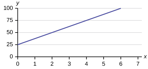
11. The y-intercept is 50 (a = 50). At the start of the cleaning, the company charges a one-time fee of $50 (this is when x = 0). The slope is 100 (b = 100). For each session, the company charges $100 for each hour they clean.
13. 12,000 pounds of soil
15. The slope is –1.5 (b = –1.5). This means the stock is losing value at a rate of $1.50 per hour. The y-intercept is $15 (a = 15). This means the price of stock before the trading day was $15.
17.
- independent variable: age; dependent variable: fatalities
- independent variable: # of family members; dependent variable: grocery bill
- independent variable: age of applicant; dependent variable: insurance premium
- independent variable: power consumption; dependent variable: utility
- independent variable: higher education (years); dependent variable: crime rates
Scatter Plots
20. The data appear to be linear with a strong, positive correlation.
22. The data appear to have no correlation.
25. For graph: check student’s solution. Note that tuition is the independent variable and salary is the dependent variable.
The Regression Equation
29. ŷ = 2.23 + 1.99x
31. The slope is 1.99 (b = 1.99). It means that for every endorsement deal a professional player gets, he gets an average of another $1.99 million in pay each year.
33. It means that there is no correlation between the data sets.
35. Yes, there are enough data points and the value of r is strong enough to show that there is a strong negative correlation between the data sets.
37. It means that 72% of the variation in the dependent variable (y) can be explained by the variation in the independent variable (x).
Testing the Significance of the Correlation Coefficient
40. Ha: ρ ≠ 0
42. We do not reject the null hypothesis. There is not sufficient evidence to conclude that there is a significant linear relationship between x and y because the correlation coefficient is not significantly different from zero.
Prediction
44. $250,120
46. 1,326 acres
48. 1,125 hours, or when x = 1,125
52.
We don’t know if the pre-1981 data was collected from a single year. So we don’t have an accurate x value for this figure.
Regression equation: ŷ (#AIDS Cases) = –3,448,225 + 1749.777 (year)
| Coefficients | |
|---|---|
| Intercept | –3,448,225 |
| X Variable 1 |
1,749.777
|
65.
-
Age Number of Driver Deaths per 100,000 16–19 38 20–24 36 25–34 24 35–54 20 55–74 18 75+ 28 - Check student’s solution.
- ŷ = 35.5818045 – 0.19182491x
- r = –0.57874
For four df and alpha = 0.05, the LinRegTTest gives p-value = 0.2288 so we do not reject the null hypothesis; there is not a significant linear relationship between deaths and age.Using the table of critical values for the correlation coefficient, with four df, the critical value is 0.811. The correlation coefficient r = –0.57874 is not less than –0.811, so we do not reject the null hypothesis.
- if age = 40, ŷ (deaths) = 35.5818045 – 0.19182491(40) = 27.9
if age = 60, ŷ (deaths) = 35.5818045 – 0.19182491(60) = 24.1
- For entire dataset, there is a linear relationship for the ages up to age 74. The oldest age group shows an increase in deaths from the prior group, which is not consistent with the younger ages.
- slope = –0.19182491
67.
- We wonder if the better discounts appear earlier in the book so we select page as X and discount as Y.
- Check student’s solution.
- ŷ = 17.21757 – 0.01412x
- r = – 0.2752
For seven df and alpha = 0.05, using LinRegTTest p-value = 0.4736 so we do not reject; there is a not a significant linear relationship between page and discount.Using the table of critical values for the correlation coefficient, with seven df, the critical value is 0.666. The correlation coefficient xi = –0.2752 is not less than 0.666 so we do not reject.
- page 10: 17.08 page 70: 16.23
- There is not a significant linear correlation so it appears there is no relationship between the page and the amount of the discount.
- page 200: 14.39
- No, using the regression equation to predict for page 200 is extrapolation.
- slope = –0.01412
As the page number increases by one page, the discount decreases by $0.01412
- Year is the independent or x variable; the number of letters is the dependent or y variable.
- Check student’s solution.
- no
- ŷ = 47.03 – 0.0216x
- –0.4280
- 6; 5
- No, the relationship does not appear to be linear; the correlation is not significant.
- current year: 2013: 3.55 or four letters; this is not an appropriate use of the least squares line. It is extrapolation.
Outliers
70. Yes, there appears to be an outlier at (6, 58).
72. The potential outlier flattened the slope of the line of best fit because it was below the data set. It made the line of best fit less accurate is a predictor for the data.
74. s = 1.75
77.
a. and b. Check student’s solution.
c. The slope of the regression line is -0.3179 with a y-intercept of 32.966. In context, the y-intercept indicates that when there are no returning sparrow hawks, there will be almost 31% new sparrow hawks, which doesn’t make sense since if there are no returning birds, then the new percentage would have to be 100% (this is an example of why we do not extrapolate). The slope tells us that for each percentage increase in returning birds, the percentage of new birds in the colony decreases by 0.3179%.
d. If we examine r2, we see that only 50.238% of the variation in the percent of new birds is explained by the model and the correlation coefficient, r = 0.71 only indicates a somewhat strong correlation between returning and new percentages.
e. The ordered pair (66, 6) generates the largest residual of 6.0. This means that when the observed return percentage is 66%, our observed new percentage, 6%, is almost 6% less than the predicted new value of 11.98%. If we remove this data pair, we see only an adjusted slope of -0.2723 and an adjusted intercept of 30.606. In other words, even though this data generates the largest residual, it is not an outlier, nor is the data pair an influential point.
f. If there are 70% returning birds, we would expect to see y = -0.2723(70) + 30.606 = 0.115 or 11.5% new birds in the colony.
79.
- Check student’s solution.
- Check student’s solution.
- We have a slope of –1.4946 with a y-intercept of 193.88. The slope, in context, indicates that for each additional minute added to the swim time, the heart rate will decrease by 1.5 beats per minute. If the student is not swimming at all, the y-intercept indicates that his heart rate will be 193.88 beats per minute. While the slope has meaning (the longer it takes to swim 2,000 meters, the less effort the heart puts out), the y-intercept does not make sense. If the athlete is not swimming (resting), then his heart rate should be very low.
- Since only 1.5% of the heart rate variation is explained by this regression equation, we must conclude that this association is not explained with a linear relationship.
- The point (34.72, 124) generates the largest residual of –11.82. This means that our observed heart rate is almost 12 beats less than our predicted rate of 136 beats per minute. When this point is removed, the slope becomes 1.6914 with the y-intercept changing to 83.694. While the linear association is still very weak, we see that the removed data pair can be considered an influential point in the sense that the y-intercept becomes more meaningful.
81. If we remove the two service academies (the tuition is $0.00), we construct a new regression equation of y = –0.0009x + 160 with a correlation coefficient of 0.71397 and a coefficient of determination of 0.50976. This allows us to say there is a fairly strong linear association between tuition costs and salaries if the service academies are removed from the data set.
83.
- Check student’s solution.
- yes
- ŷ = −266.8863+0.1656x
- 0.9448; Yes
- 62.8233; 62.3265
- yes
- yes; (1987, 62.7)
- 72.5937; no
- slope = 0.1656.
As the year increases by one, the percent of workers paid hourly rates tends to increase by 0.1656.
85.
| Size (ounces) | Cost ($) | cents/oz |
|---|---|---|
| 16 | 3.99 | 24.94 |
| 32 | 4.99 | 15.59 |
| 64 | 5.99 | 9.36 |
| 200 | 10.99 | 5.50 |
Check student’s solution.
There is a linear relationship for the sizes 16 through 64, but that linear trend does not continue to the 200-oz size.
ŷ = 20.2368 – 0.0819x
r = –0.8086
40-oz: 16.96 cents/oz
90-oz: 12.87 cents/oz
The relationship is not linear; the least squares line is not appropriate.
no outliers
No, you would be extrapolating. The 300-oz size is outside the range of x.
slope = –0.08194; for each additional ounce in size, the cost per ounce decreases by 0.082 cents.
87.
- Size is x, the independent variable, price is y, the dependent variable.
- Check student’s solution.
- The relationship does not appear to be linear.
- ŷ = –745.252 + 54.75569x
- r = 0.8944, yes it is significant
- 32-inch: $1006.93, 50-inch: $1992.53
- No, the relationship does not appear to be linear. However, r is significant.
- yes, the 60-inch TV
- For each additional inch, the price increases by $54.76
89.
- Let rank be the independent variable and area be the dependent variable.
- Check student’s solution.
- There appears to be a linear relationship, with one outlier.
- ŷ (area) = 24177.06 + 1010.478x
- r = 0.50047, r is not significant so there is no relationship between the variables.
- Alabama: 46407.576 Colorado: 62575.224
- Alabama estimate is closer than Colorado estimate.
- If the outlier is removed, there is a linear relationship.
- There is one outlier (Hawaii).
- rank 51: 75711.4; no
-
Alabama 7 1819 22 52,423 Colorado 8 1876 38 104,100 Alaska 6 1959 51 656,424 Iowa 4 1846 29 56,276 Maryland 8 1788 7 12,407 Missouri 8 1821 24 69,709 New Jersey 9 1787 3 8,722 Ohio 4 1803 17 44,828 South Carolina 13 1788 8 32,008 Utah 4 1896 45 84,904 Wisconsin 9 1848 30 65,499 - ŷ = –87065.3 + 7828.532x
- Alabama: 85,162.404; the prior estimate was closer. Alaska is an outlier.
- yes, with the exception of Hawaii
Candela Citations
- Introductory Statistics . Authored by: Barbara Illowski, Susan Dean. Provided by: Open Stax. Located at: http://cnx.org/contents/30189442-6998-4686-ac05-ed152b91b9de@17.44. License: CC BY: Attribution. License Terms: Download for free at http://cnx.org/contents/30189442-6998-4686-ac05-ed152b91b9de@17.44