Equilibrium, Surplus, and Shortage

Demand and Supply
In order to understand market equilibrium, we need to start with the laws of demand and supply. Recall that the law of demand says that as price decreases, consumers demand a higher quantity. Similarly, the law of supply says that when price decreases, producers supply a lower quantity.
Because the graphs for demand and supply curves both have price on the vertical axis and quantity on the horizontal axis, the demand curve and supply curve for a particular good or service can appear on the same graph. Together, demand and supply determine the price and the quantity that will be bought and sold in a market. These relationships are shown as the demand and supply curves in Figure 1, which is based on the data in Table 1, below.
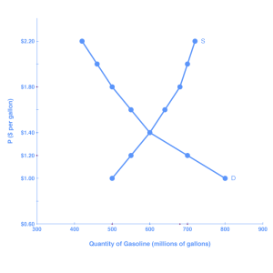
Figure 1. Demand and Supply for Gasoline
Table 1. Price, Quantity Demanded, and Quantity Supplied
| Price (per gallon) | Quantity demanded (millions of gallons) | Quantity supplied (millions of gallons) |
|---|---|---|
| $1.00 | 800 | 500 |
| $1.20 | 700 | 550 |
| $1.40 | 600 | 600 |
| $1.60 | 550 | 640 |
| $1.80 | 500 | 680 |
| $2.00 | 460 | 700 |
| $2.20 | 420 | 720 |
If you look at either Figure 1 or Table 1, you’ll see that, at most prices, the amount that consumers want to buy (which we call quantity demanded) is different from the amount that producers want to sell (which we call quantity supplied). What does it mean when the quantity demanded and the quantity supplied aren’t the same? Answer: a surplus or a shortage.
Surplus or Excess Supply
Let’s consider one scenario in which the amount that producers want to sell doesn’t match the amount that consumers want to buy. Suppose that a market produces more than the quantity demanded. Let’s use our example of the price of a gallon of gasoline. Imagine that the price of a gallon of gasoline were $1.80 per gallon. This price is illustrated by the dashed horizontal line at the price of $1.80 per gallon in Figure 2, below.
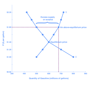
Figure 2. Demand and Supply for Gasoline: Surplus
At this price, the quantity demanded is 500 gallons, and the quantity of gasoline supplied is 680 gallons. You can also find these numbers in Table 1, above. Now, compare quantity demanded and quantity supplied at this price. Quantity supplied (680) is greater than quantity demanded (500). Or, to put it in words, the amount that producers want to sell is greater than the amount that consumers want to buy. We call this a situation of excess supply (since Qs > Qd) or a surplus. Note that whenever we compare supply and demand, it’s in the context of a specific price—in this case, $1.80 per gallon.
With a surplus, gasoline accumulates at gas stations, in tanker trucks, in pipelines, and at oil refineries. This accumulation puts pressure on gasoline sellers. If a surplus remains unsold, those firms involved in making and selling gasoline are not receiving enough cash to pay their workers and cover their expenses. In this situation, some producers and sellers will want to cut prices, because it is better to sell at a lower price than not to sell at all. Once some sellers start cutting prices, others will follow to avoid losing sales. These price reductions will, in turn, stimulate a higher quantity demanded.
How far will the price fall? Whenever there is a surplus, the price will drop until the surplus goes away. When the surplus is eliminated, the quantity supplied just equals the quantity demanded—that is, the amount that producers want to sell exactly equals the amount that consumers want to buy. We call this equilibrium, which means “balance.” In this case, the equilibrium occurs at a price of $1.40 per gallon and at a quantity of 600 gallons. You can see this in Figure 2 (and Figure 1) where the supply and demand curves cross. You can also find it in Table 1 (the numbers in bold).
Equilibrium: Where Supply and Demand Intersect
When two lines on a diagram cross, this intersection usually means something. On a graph, the point where the supply curve (S) and the demand curve (D) intersect is the equilibrium. The equilibrium price is the only price where the desires of consumers and the desires of producers agree—that is, where the amount of the product that consumers want to buy (quantity demanded) is equal to the amount producers want to sell (quantity supplied). This mutually desired amount is called the equilibrium quantity. At any other price, the quantity demanded does not equal the quantity supplied, so the market is not in equilibrium at that price.
If you have only the demand and supply schedules, and no graph, you can find the equilibrium by looking for the price level on the tables where the quantity demanded and the quantity supplied are equal (again, the numbers in bold in Table 1 indicate this point).
FINDING EQUILIBRIUM WITH ALGEBRA
We’ve just explained two ways of finding a market equilibrium: by looking at a table showing the quantity demanded and supplied at different prices, and by looking at a graph of demand and supply. We can also identify the equilibrium with a little algebra if we have equations for the supply and demand curves.
Let’s practice solving a few equations that you will see later in the course. Right now, we are only going to focus on the math. Later you’ll learn why these models work the way they do, but let’s start by focusing on solving the equations.
Suppose that the demand for soda is given by the following equation:
[latex]Qd=16–2P\\[/latex]
where Qd is the amount of soda that consumers want to buy (i.e., quantity demanded), and P is the price of soda.
Suppose the supply of soda is
[latex]Qs=2+5P\\[/latex]
where Qs is the amount of t that producers will supply (i.e., quantity supplied).
Finally, suppose that the soda market operates at a point where supply equals demand, or
[latex]Qd=Qs\\[/latex]
We now have a system of three equations and three unknowns (Qd, Qs, and P), which we can solve with algebra. Since [latex]Qd=Qs\\[/latex], we can set the demand and supply equation equal to each other:
[latex]\begin{array}{c}\,\,Qd=Qs\\16-2P=2+5P\end{array}\\[/latex]
Step 1: Isolate the variable by adding 2P to both sides of the equation, and subtracting 2 from both sides.
[latex]\begin{array}{l}\,16-2P=2+5P\\-2+2P=-2+2P\\\,\,\,\,\,\,\,\,\,\,\,\,\,\,\,14=7P\end{array}\\[/latex]
Step 2: Simplify the equation by dividing both sides by 7.
[latex]\begin{array}{l}\underline{14}=\underline{7P}\\\,\,\,7\,\,\,\,\,\,\,\,\,\,7\\\,\,\,\,2=P\end{array}\\[/latex]
The price of each soda will be $2. Now we want to understand the amount of soda that consumers want to buy, or the quantity demanded, at a price of $2.
Remember, the formula for quantity demanded is the following:
[latex]Qd=16-2P\\[/latex]
Taking the price of $2, and plugging it into the demand equation, we get
[latex]\begin{array}{l}Qd=16–2(2)\\Qd=16–4\\Qd=12\end{array}[/latex]
So, if the price is $2 each, consumers will purchase 12. How much will producers supply, or what is the quantity supplied? Taking the price of $2, and plugging it into the equation for quantity supplied, we get the following:
[latex]\begin{array}{l}Qs=2+5P\\Qs=2+5(2)\\Qs=2+10\\Qs=12\end{array}\\[/latex]
Now, if the price is $2 each, producers will supply 12 sodas. This means that we did our math correctly, since [latex]Qd=Qs\\[/latex] and both Qd and Qs are equal to 12.
Shortage or Excess Demand
Let’s return to our gasoline problem. Suppose that the price is $1.20 per gallon, as the dashed horizontal line at this price in Figure 3, below, shows. At this price, the quantity demanded is 700 gallons, and the quantity supplied is 550 gallons.
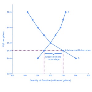
Figure 3. Demand and Supply for Gasoline: Shortage
Quantity supplied (550) is less than quantity demanded (700). Or, to put it in words, the amount that producers want to sell is less than the amount that consumers want to buy. We call this a situation of excess demand (since Qd > Qs) or a shortage.
In this situation, eager gasoline buyers mob the gas stations, only to find many stations running short of fuel. Oil companies and gas stations recognize that they have an opportunity to make higher profits by selling what gasoline they have at a higher price. These price increases will stimulate the quantity supplied and reduce the quantity demanded. As this occurs, the shortage will decrease. How far will the price rise? The price will rise until the shortage is eliminated and the quantity supplied equals quantity demanded. In other words, the market will be in equilibrium again. As before, the equilibrium occurs at a price of $1.40 per gallon and at a quantity of 600 gallons.
Generally any time the price for a good is below the equilibrium level, incentives built into the structure of demand and supply will create pressures for the price to rise. Similarly, any time the price for a good is above the equilibrium level, similar pressures will generally cause the price to fall.
As you can see, the quantity supplied or quantity demanded in a free market will correct over time to restore balance, or equilibrium.
Equilibrium and Economic Efficiency
Equilibrium is important to create both a balanced market and an efficient market. If a market is at its equilibrium price and quantity, then it has no reason to move away from that point, because it’s balancing the quantity supplied and the quantity demanded. However, if a market is not at equilibrium, then economic pressures arise to move the market toward the equilibrium price and equilibrium quantity. This happens either because there is more supply than what the market is demanding or because there is more demand than the market is supplying. This balance is a natural function of a free-market economy.
Also, a competitive market that is operating at equilibrium is an efficient market. Economist typically define efficiency in this way: when it is impossible to improve the situation of one party without imposing a cost on another. Conversely, if a situation is inefficient, it becomes possible to benefit at least one party without imposing costs on others.
Efficiency in the demand and supply model has the same basic meaning: The economy is getting as much benefit as possible from its scarce resources, and all the possible gains from trade have been achieved. In other words, the optimal amount of each good and service is being produced and consumed.

Figure 4. Demand and Supply for Gasoline: Equilibrium
Equilibrium occurs at the point where quantity supplied = quantity demanded.
Changes in Equilibrium

The Four-Step Process
Let’s begin this discussion with a single economic event. It might be an event that affects demand, like a change in income, population, tastes, prices of substitutes or complements, or expectations about future prices. It might be an event that affects supply, like a change in natural conditions, input prices, technology, or government policies that affect production. How does an economic event like one of these affect equilibrium price and quantity? We’ll investigate this question using a four-step process.
Step 1. Draw a demand and supply model before the economic change took place. Creating the model requires four standard pieces of information: the law of demand, which tells us the slope of the demand curve; the law of supply, which gives us the slope of the supply curve; the shift variables for demand; and the shift variables for supply. From this model, find the initial equilibrium values for price and quantity.
Step 2. Decide whether the economic change being analyzed affects demand or supply. In other words, does the event refer to something in the list of demand factors or supply factors?
Step 3. Decide whether the effect on demand or supply causes the curve to shift to the right or to the left, and sketch the new demand or supply curve on the diagram. In other words, does the event increase or decrease the amount consumers want to buy or producers want to sell?
Step 4. Identify the new equilibrium, and then compare the original equilibrium price and quantity to the new equilibrium price and quantity.
Newspapers and the Internet
According to the Pew Research Center for People and the Press, more and more people, especially younger people, are getting their news from online and digital sources. The majority of U.S. adults now own smartphones or tablets, and most of those Americans say they use them in part to get the news. From 2004 to 2012, the share of Americans who reported getting their news from digital sources increased from 24 percent to 39 percent. How has this trend affected consumption of print news media and radio and television news? Figure 1 and the text below illustrate the four-step analysis used to answer this question.
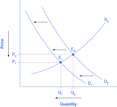
Figure 1. The Print News Market: A Four-Step Analysis
Step 1. Develop a demand and supply model to think about what the market looked like before the event. The demand curve D0 and the supply curve S0 show the original relationships. In this case, the analysis is performed without specific numbers on the price and quantity axis.
Step 2. Did the change described affect supply or demand? A change in tastes, from traditional news sources (print, radio, and television) to digital sources, caused a change in demand for the former.
Step 3. Was the effect on demand positive or negative? A shift to digital news sources will tend to mean a lower quantity demanded of traditional news sources at every given price, causing the demand curve for print and other traditional news sources to shift to the left, from D0 to D1.
Step 4. Compare the new equilibrium price and quantity to the original equilibrium price. The new equilibrium (E1) occurs at a lower quantity and a lower price than the original equilibrium (E0).
The decline in print news reading predates 2004. Print newspaper circulation peaked in 1973 and has declined since then due to competition from television and radio news. In 1991, 55 percent of Americans indicated that they got their news from print sources, while only 29 percent did so in 2012. Radio news has followed a similar path in recent decades, with the share of Americans getting their news from radio declining from 54 percent in 1991 to 33 percent in 2012. Television news has held its own during the last fifteen years, with the market share staying in the mid to upper fifties. What does this suggest for the future, given that two-thirds of Americans under thirty years old say they don’t get their news from television at all?
Worked Example: Supply and Demand
The example we just considered showed a shift to the left in the demand curve, as a change in consumer preferences reduced demand for newspapers. Often changes in an economy affect both the supply and the demand curves, making it more difficult to assess the impact on the equilibrium price. Let’s review one such example.
First, consider the following questions:

- Suppose postal workers are successful in obtaining a pay raise from the U.S. Postal Service. Will this affect the supply or the demand for first-class mail? Why? Which determinant of demand or supply is being affected? Show graphically with before and after curves on the same axes. How will this change the equilibrium price and quantity of first-class mail?
- How do you imagine the invention of email and text messaging affected the market for first-class mail? Why? Which determinant of demand or supply is being affected? Show graphically with before and after curves on the same axes. How will this change the equilibrium price and quantity of first-class mail?
- Suppose that postal workers get a pay raise and email and text messaging become common. What will the combined impact be on the equilibrium price and quantity of first-class mail?
In order to complete a complex analysis like this it’s helpful to tackle the parts separately and then combine them, while thinking about possible interactions between the two parts that might affect the overall outcome.
Part 1: A Pay Raise for Postal Workers
A pay raise for postal workers would represent an increase in the cost of production for the Postal Service. Production costs are a factor that influences supply; thus, the pay raise should decrease the supply of first-class mail, shifting the supply curve vertically by the amount of the pay raise. Intuitively, all else held constant, the Postal Service would like to charge a higher price that incorporates the higher cost of production. That is not to say the higher price will stick. From the graph (Figure 1), it should be clear that at that higher price, the quantity supplied is greater than the quantity demanded—thus there would be a surplus, indicating that the price the Postal Service desires is not an equilibrium price. Or to put it differently, at the original price (P1), the decrease in supply causes a shortage driving up the price to a new equilibrium level (P2). Note that the price doesn’t rise by the full amount of the pay increase. In short, a leftward shift in the supply curve causes a movement up the demand curve, resulting in a lower equilibrium quantity (Q2) and a higher equilibrium price (P2).

Figure 1
Part 2: The Effect of Email and Text Messaging
Since many people find email and texting more convenient than sending a letter, we can assume that tastes and preferences for first-class mail will decline. This decrease in demand is shown by a leftward shift in the demand curve and a movement along the supply curve, which creates a surplus in first-class mail at the original price (shown as P2). The shortage causes a decrease in the equilibrium price (to P3) and a decrease in the equilibrium quantity (to Q3). Intuitively, less demand for first-class mail leads to a lower equilibrium quantity and (ceteris paribus) a lower equilibrium price.

Figure 2
Part 3: Combining Factors
Parts 1 and 2 are straightforward, but when we put them together it becomes more complex. Think about it this way: In Part 1, the equilibrium quantity fell due to decreased supply. In Part 2, the equilibrium quantity also fell, this time due to the decreased demand. So putting the two parts together, we would expect to see the final equilibrium quantity (Q3) to be smaller than the original equilibrium quantity (Q1). So far, so good.
Now consider what happens to the price. In Part 1, the equilibrium price increased due to the reduction in supply. But in Part 2, the equilibrium price decreased due to the decrease in demand! What will happen to the equilibrium price? The net effect on price can’t be determined without knowing which curve shifts more, demand or supply. The equilibrium price could increase, decrease, or stay the same. You just can’t tell from graphical analysis alone.

Figure 3
Try It: Food Trucks and Changes in Equilibrium
Play the simulation below multiple times to see how different choices lead to different outcomes. All simulations allow unlimited attempts so that you can gain experience applying the concepts.
Problem Sets: Supply and Demand
Test your understanding of the learning outcomes in this module by working through the following problems. These problems aren’t graded, but they give you a chance to practice before taking the quiz.
If you’d like to try a problem again, you can click the link that reads, “Try another version of these questions.”
Use the information provided in the first question for all of the questions in this problem set.
Check Your Understanding
Answer the question(s) below to see how well you understand the topics covered above. This short quiz does not count toward your grade in the class, and you can retake it an unlimited number of times.
Use this quiz to check your understanding and decide whether to (1) study the previous section further or (2) move on to the next section.
Candela Citations
- Revision and adaptation. Authored by: Linda Williams and Lumen Learning. License: CC BY: Attribution
- Food Trucks and Changes in Equilibrium. Authored by: Clark Aldridge for Lumen Learning. License: CC BY: Attribution
- Problem Sets: Supply and Demand. Provided by: Lumen Learning. License: CC BY: Attribution
- Check Your Understanding. Authored by: Lumen Learning. License: CC BY: Attribution
- Demand, Supply, and Equilibrium in Markets for Goods and Services. Authored by: OpenStax College. Provided by: Rice University. Located at: https://cnx.org/contents/D3bzsNhU@8/Demand-Supply-and-Equilibrium-. License: CC BY: Attribution
- Episode 14: Market Equilibrium. Authored by: Dr. Mary J. McGlasson. Located at: https://youtu.be/W5nHpAn6FvQ?t=1s. License: CC BY-NC-ND: Attribution-NonCommercial-NoDerivatives
- Principles of Macroeconomics Chapter 3.3. Authored by: OpenStax College. Provided by: Rice University. Located at: http://cnx.org/contents/ea2f225e-6063-41ca-bcd8-36482e15ef65@10.31:24/Microeconomics. License: CC BY: Attribution
- Newspaper forest green. Authored by: Jon S. Located at: https://www.flickr.com/photos/62693815@N03/6277389273/. License: CC BY: Attribution
- From Eagle to Snail. Authored by: dalioPhoto. Located at: https://www.flickr.com/photos/marcdalio/7771613398/. License: CC BY-NC-ND: Attribution-NonCommercial-NoDerivatives