Learning Objectives
- Estimate the probability of an event using a normal model of the sampling distribution.
Let’s compare what we have learned about sampling distributions for proportions and for means.
| Sampling Distribution | |||||
|---|---|---|---|---|---|
| Variable | Parameter | Statistic | Center | Spread | Shape |
| Categorical (example: left-handed or not) | p = population proportion | [latex]\stackrel{ˆ}{p}[/latex] = sample proportion | p | [latex]\sqrt{\frac{p(1-p)}{n}}[/latex] | Normal if np ≥ 10 and n(1 – p) ≥ 10 |
| Quantitative (example: age) | μ = population mean, σ = population standard deviation | [latex]\overline{x}[/latex] = sample mean | μ | [latex]\frac{\sigma }{\sqrt{n}}[/latex] | Normal if n > 30 (always normal if population is normal) |
Now we know the conditions that allow us to use a normal model for the sampling distribution of means. As we have done before, we now convert sample means to z-scores and use a standard normal curve to find probabilities and identify unusual sample means.
Normal Model Simulation Useful Again
Recall the standard normal model simulation we first used in Probability and Probability Distribution. It was our tool for converting between intervals of z-scores and probabilities.
Click here to open this simulation in its own window.
Example
Surprising Heights for Individual Basketball Players
Suppose we have a population of adult male basketball players and we know their heights: the mean height is μ = 190 cm and the standard deviation of their heights is σ = 7.2 cm. The heights are normally distributed, which is often the case with body measurements.
Would it be surprising to find a randomly chosen player from this population with a height of 195 cm?
We can answer this question by computing the probability that a randomly chosen player from this population has height greater than 195 cm. To carry out the analysis, let’s use X to denote the height of a randomly chosen individual from this population. Since heights are normally distributed, we can convert heights to z-scores and use our simulation to find the probability P(X > 195).
- Convert the interval X > 195 to an interval of z-scores.Recall that the z-score of an X-value is the number of standard deviations that value is away from the mean. The formula is
[latex]Z\text{}=\text{}\frac{X-μ}{σ}[/latex]
So the z-score of X = 195 is
[latex]\frac{X-μ}{σ}\text{}=\text{}\frac{195-190}{7.2}\text{}=\text{}\frac{5}{7.2}\text{}=\text{}0.69[/latex]
That means that the interval of X-values “X > 195” corresponds to the interval of Z-values “Z > 0.69.”
- Convert the interval Z > 0.69 to a probability statement.We use the simulation (or some sort of technology) for this step. Below is a picture of the simulation with the settings for this problem. We moved one flag out of the way and the other flag to the position Z = 0.69. For a “greater than” probability, we want the area to the right of Z = 0.69.
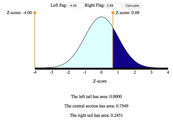
So we have found that P(X > 195) = P(Z > 0.69) = 0.2451.
Conclusion: This probability is not very low (almost 25%). We conclude that it would be not be surprising to find a randomly chosen individual from this population with a height of 195 cm.
Example
Surprising Heights for Samples of Basketball Players
As before, suppose the heights of individual players are normally distributed with μ = 190 cm and σ = 7.2 cm.
Would it be surprising to find a randomly chosen team of 25 players with a mean height of 195 cm?
We compute the probability that a random sample of 25 players has a mean height of 195 cm or more. We have to look at the distribution of all sample means for samples of size 25. Here’s what we know about this sampling distribution:
- The distribution of sample means is normal, even though our sample size is less than 30, because we know the distribution of individual heights is normal. If the individual heights were not normally distributed, we would need a larger sample size before using a normal model for the sampling distribution.
- The mean of the sampling distribution is 195 cm, the same as the mean of the individual heights.
- The standard deviation of the sampling distribution is[latex]\mathrm{σ}\text{}/\sqrt{n}\text{}=\text{}7.2\text{}/\sqrt{25}\text{}=\text{}7.2\text{}/\text{}5\text{}=\text{}1.44[/latex]
Now we can answer this question by computing the probability that a randomly chosen sample of 25 players from this population has mean height greater than 195 cm. To carry out the analysis, let’s use [latex]\overline{X}[/latex] to denote the mean height of a random sample of 25 players from this population. Because mean heights are normally distributed, we can convert mean heights to z-scores and use our simulation to find the probability P( [latex]\overline{X}[/latex] > 195).
- Convert the interval [latex]\overline{X}[/latex] > 195 to an interval of z-scores.Note that the z-score is the number of standard errors the sample mean is from µ. So the z-score calculation for the sampling distribution has mean μ = 190 and standard deviation [latex]\mathrm{σ}\text{}/\sqrt{n}\text{}=\text{}1.44[/latex].The formula for the z-score of [latex]\overline{X}[/latex] is
[latex]Z\text{}=\text{}\frac{\stackrel{¯}{X}-\mathrm{μ}}{\mathrm{σ}\text{}/\sqrt{n}}[/latex]
So the z-score of [latex]\overline{X}[/latex] = 195 is
[latex]\frac{\stackrel{¯}{X}-\mathrm{μ}}{\mathrm{σ}\text{}/\sqrt{n}}\text{}=\text{}\frac{195-190}{1.44}\text{}=\text{}\frac{5}{1.44}\text{}=\text{}3.47[/latex]
And the interval of [latex]\overline{X}[/latex]-values “[latex]\overline{X}[/latex] > 195” corresponds to the interval of Z-values “Z > 3.47.”
- Convert the interval Z > 3.47 to a probability statement.Again, we use the simulation as we did in the previous example. Move the left-hand flag out of the way and the right-hand flag to Z = 3.47. For a “greater than” probability, we want the area to the right of Z = 3.47.
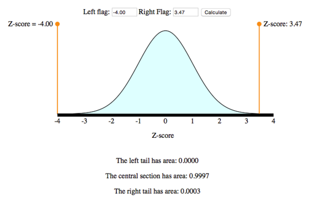
So we have found that [latex]P(\stackrel{¯}{X}>195)\text{}=\text{}P(Z>3.47)\text{}=\text{}0.0003[/latex].
Conclusion: This probability is very low (much, much less than 1%). We conclude that it would be very surprising to find a random sample of 25 players from this population with a mean height of 195 cm.
It’s interesting to notice that the height cutoff we used in these two examples is the same (195 cm). When considering the individual, we concluded that finding a randomly chosen individual with height of 195 cm would not be surprising. However, when we considered the team, we concluded that it would be very surprising to find a random sample of 25 players with a mean height of 195 cm. This makes sense because as sample size grows, variability shrinks (here we considered a sample of size 1 versus a sample of size 25).
Click here to open the normal simulation in a separate window to answer the following questions.
Learn By Doing
The annual salary of teachers in a certain state X has a mean of μ = $54,000 and standard deviation of σ = $5,000.
What Have We Learned Here?
We need to be careful before using the normal model to find probabilities associated with sample means.
- If the individual values are normally distributed, then the sampling distribution of means will be normal for any sample size. In this case, we can use the normal model to compute probabilities without worrying about the sample size.
- On the other hand, if the individual values are not normally distributed, then we have to make sure the sample size is large enough before concluding that the sampling distribution of means is approximately normal. The general rule is that the sample size should be more than 30 in order for us to feel confident that the sampling distribution of means is approximately normal (but it really depends on the shape of the distribution of individual values).
Note: The logic of inference in this module is familiar. We make a claim about a population mean. We use a random sample to test our claim. We determine whether it is probable that random samples have means as extreme as the actual sample. If this is very unlikely, then we conclude this sample probably could not have come from this population and that the claim about the population mean is probably false. We used logic like this in Modules 7, 8, and 9 in the context of proportions. In this module, we further develop this idea in the context of means.
Let’s Summarize
- Many questions regarding quantitative variables require us to say something about the mean of a large population. It is often necessary to compute statistics from a random sample and use them to make an estimate or an inference about the population mean.
- We need to be able to compute the probability that the mean of a random sample falls in a given range. This probability allows us to draw an inference about the population parameter. To compute this probability, we need to understand the distribution of all sample means.
- Let’s say we have a quantitative data set from a population with mean µ and standard deviation σ. The model for the theoretical sampling distribution of means of all random samples of size n has the following properties:
- The mean of the sampling distribution of means is µ.
- The standard deviation of the sampling distribution of means is [latex]σ\text{}/\sqrt{n}[/latex].
- Notice that as n grows, the standard deviation of the sampling distribution of means shrinks. It means that larger samples give more accurate estimates of population means.
- The central limit theorem states that for large enough sample sizes, the sampling distribution of means is approximately normal, even if the population is not normal.
- If a variable has a skewed distribution for individuals in the population, a larger sample size is needed to ensure that the sampling distribution has a normal shape.
- The general rule is that if n is more than 30, the sampling distribution of means will be approximately normal. However, if the population is already normal, then any sample size will produce a normal sampling distribution.
- The mechanics of finding a probability associated with a range of sample means usually proceeds as follows.
- Convert a sample mean [latex]\stackrel{¯}{X}[/latex] into a z-score: [latex]Z\text{}=\text{}\frac{\stackrel{¯}{X}-μ}{σ/\sqrt{n}}[/latex].
- Use technology to find a probability associated with a given range of z-scores.
Candela Citations
- Concepts in Statistics. Provided by: Open Learning Initiative. Located at: http://oli.cmu.edu. License: CC BY: Attribution