Cost behavior patterns
There are four basic cost behavior patterns: fixed, variable, mixed (semivariable), and step which graphically would appear as below.

The relevant range is the range of production or sales volume over which the assumptions about cost behavior are valid. Often, we describe them as time-related costs.
A graph depicting the relevant range would look like this:

Fixed costs remain constant (in total) over some relevant range of output. Depreciation, insurance, property taxes, and administrative salaries are examples of fixed costs. Recall that so-called fixed costs are fixed in the short run but not necessarily in the long run.
For example, a local high-tech company did not lay off employees during a recent decrease in business volume because the management did not want to hire and train new people when business picked up again. Management treated direct labor as a fixed cost in this situation. Although volume decreased, direct labor costs remained fixed.
In contrast to fixed costs, variable costs vary (in total) directly with changes in volume of production or sales. In particular, total variable costs change as total volume changes. If pizza production increases from 100 10-inch pizzas to 200 10-inch pizzas per day, the amount of dough required per day to make 10-inch pizzas would double. The dough is a variable cost of pizza production. Direct materials and sales commissions are variable costs.
Direct labor is a variable cost in many cases. If the total direct labor cost increases as the volume of output increases and decreases as volume decreases, direct labor is a variable cost. Piecework pay is an excellent example of direct labor as a variable cost. In addition, direct labor is frequently a variable cost for workers paid on an hourly basis, as the volume of output increases, more workers are hired. However, sometimes the nature of the work or management policy does not allow direct labor to change as volume changes and direct labor can be a fixed cost.
Mixed costs have both fixed and variable characteristics. A mixed cost contains a fixed portion of cost incurred even when the facility is idle, and a variable portion that increases directly with volume. Electricity is an example of a mixed cost. A company must incur a certain cost for basic electrical service. As the company increases its volume of activity, it runs more machines and runs them longer. The firm also may extend its hours of operation. As activity increases, so does the cost of electricity.
Managers usually separate mixed costs into their fixed and variable components for decision-making purposes. They include the fixed portion of mixed costs with other fixed costs, while assuming the variable part changes with volume. We will look at ways to separate fixed and variable components of a mixed cost later in the chapter.
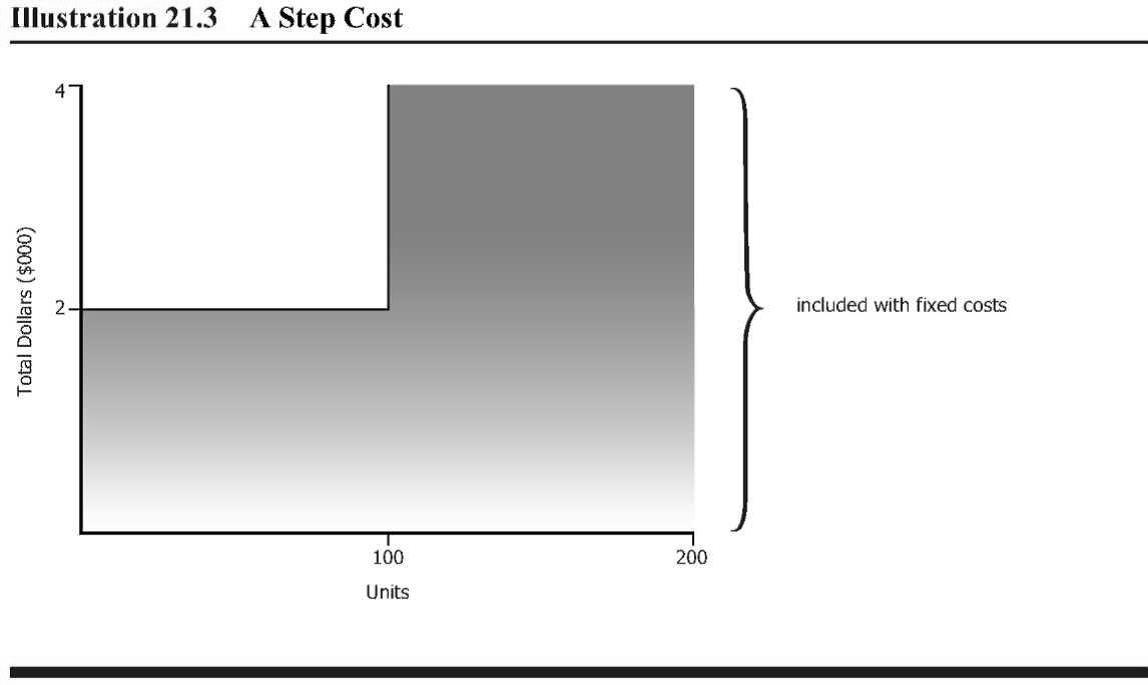
A step cost remains constant at a certain fixed amount over a range of output (or sales). Then, at certain points, the step costs increase to higher amounts. Visually, step costs appear like stair steps.
Supervisors’ salaries are an example of a step cost when companies hire additional supervisors as production increases. For instance, the local McDonald’s restaurant has one supervisor until sales exceed 100 meals during the lunch hour. If sales regularly exceed 100 meals during that hour, the company adds a second supervisor. The supervisor costs will remain the same for between 0 – 100 meals served that hour. When meals served are between 101 – 200, the supervisor cost goes up to reflect 2 supervisors. Step costs will increase by the same amount for each new cost or step. Step costs are sometimes labeled as step variable costs (many small steps) or step fixed costs (only a few large steps). In graph form, a step cost would appear as:
Although we have described four different cost patterns (fixed, variable, mixed, and step), we simplify our discussions in this chapter by assuming managers can separate mixed and step costs into fixed and variable components using cost estimation techniques.
Many costs do not vary in a strictly linear relationship with volume. Rather, costs may vary in a curvilinear pattern—a 10% increase in volume may yield an 8% change in total variable costs at lower output levels and an 11% change in total variable costs at higher output levels. We show a curvilinear cost pattern below.

One way to deal with a curvilinear cost pattern is to assume a linear relationship between costs and volume within some relevant range. Within that relevant range, the total cost varies linearly with volume, at least approximately. Outside of the relevant range, we presume the assumptions about cost behavior may be invalid.
Costs rarely behave in the simple way that would make life easy for decision makers. Even within the relevant range, the assumed cost behavior is usually only approximately linear. As decision makers, we have to live with the fact that cost estimates are not as precise as physical or engineering measurements.
Candela Citations
- Accounting Principles: A Business Perspective.. Authored by: James Don Edwards, University of Georgia & Roger H. Hermanson, Georgia State University.. Provided by: Endeavour International Corporation. Project: The Global Text Project. License: CC BY: Attribution
- What is the Relevant Range (Managerial Accounting Tutorial #4). Authored by: Note Pirate. Located at: https://youtu.be/KCpRAgs-yMw. License: All Rights Reserved. License Terms: Standard YouTube License
- Step Variable Costs. Authored by: Education Unlocked. Located at: https://youtu.be/wrmNwHAidVo. License: All Rights Reserved. License Terms: Standard YouTube License