Previously, we have tested hypotheses about two population means. This chapter examines methods for comparing more than two means. Analysis of variance (ANOVA) is an inferential method used to test the equality of three or more population means.
H0: µ1= µ2= µ3= …=µk
This method is also referred to as single-factor ANOVA because we use a single property, or characteristic, for categorizing the populations. This characteristic is sometimes referred to as a treatment or factor.
A treatment (or factor) is a property, or characteristic, that allows us to distinguish the different populations from one another.
The objects of ANOVA are (1) estimate treatment means, and the differences of treatment means; (2) test hypotheses for statistical significance of comparisons of treatment means, where “treatment” or “factor” is the characteristic that distinguishes the populations.
For example, a biologist might compare the effect that three different herbicides may have on seed production of an invasive species in a forest environment. The biologist would want to estimate the mean annual seed production under the three different treatments, while also testing to see which treatment results in the lowest annual seed production. The null and alternative hypotheses are:
| H0: µ1= µ2= µ3 | H1: at least one of the means is significantly different from the others |
It would be tempting to test this null hypothesis H0: µ1= µ2= µ3 by comparing the population means two at a time. If we continue this way, we would need to test three different pairs of hypotheses:
| H0: µ1= µ2 | AND | H0: µ1= µ3 | AND | H0: µ2= µ3 |
| H1: µ1≠ µ2 | H1: µ1≠ µ3 | H1: µ2≠ µ3 |
If we used a 5% level of significance, each test would have a probability of a Type I error (rejecting the null hypothesis when it is true) of α = 0.05. Each test would have a 95% probability of correctly not rejecting the null hypothesis. The probability that all three tests correctly do not reject the null hypothesis is 0.953 = 0.86. There is a 1 – 0.953 = 0.14 (14%) probability that at least one test will lead to an incorrect rejection of the null hypothesis. A 14% probability of a Type I error is much higher than the desired alpha of 5% (remember: α is the same as Type I error). As the number of populations increases, the probability of making a Type I error using multiple t-tests also increases. Analysis of variance allows us to test the null hypothesis (all means are equal) against the alternative hypothesis (at least one mean is different) with a specified value of α.
The assumptions for ANOVA are (1) observations in each treatment group represents a random sample from that population; (2) each of the populations is normally distributed; (3) population variances for each treatment group are homogeneous (i.e., 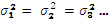 ). We can easily test the normality of the samples by creating a normal probability plot, however, verifying homogeneous variances can be more difficult. A general rule of thumb is as follows: One-way ANOVA may be used if the largest sample standard deviation is no more than twice the smallest sample standard deviation.
In the previous chapter, we used a two-sample t-test to compare the means from two independent samples with a common variance. The sample data are used to compute the test statistic:
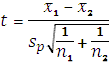 where
where 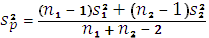
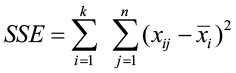
is the pooled estimate of the common population variance σ2. To test more than two populations, we must extend this idea of pooled variance to include all samples as shown below:
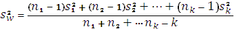
where Sw2 represents the pooled estimate of the common variance σ2, and it measures the variability of the observations within the different populations whether or not H0 is true. This is often referred to as the variance within samples (variation due to error).
If the null hypothesis IS true (all the means are equal), then all the populations are the same, with a common mean μ and variance σ2. Instead of randomly selecting different samples from different populations, we are actually drawing k different samples from one population. We know that the sampling distribution for k means based on n observations will have mean μx̄ and variance σ2/n (squared standard error). Since we have drawn k samples of n observations each, we can estimate the variance of the k sample means (σ2/n) by
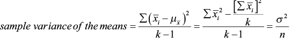
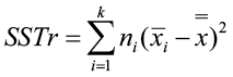
Consequently, n times the sample variance of the means estimates σ2. We designate this quantity as SB2 such that
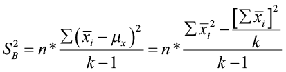
where SB2 is also an unbiased estimate of the common variance σ2, IF H0 IS TRUE. This is often referred to as the variance between samples (variation due to treatment).
Under the null hypothesis that all k populations are identical, we have two estimates of σ2 (SW2 and SB2). We can use the ratio of SB2/ SW2 as a test statistic to test the null hypothesis that H0: µ1= µ2= µ3= …= µk, which follows an F-distribution with degrees of freedom df1= k – 1 and df2 = N – k (where k is the number of populations and N is the total number of observations (N = n1 + n2+…+ nk). The numerator of the test statistic measures the variation between sample means. The estimate of the variance in the denominator depends only on the sample variances and is not affected by the differences among the sample means.
When the null hypothesis is true, the ratio of SB2 and SW2 will be close to 1. When the null hypothesis is false, SB2 will tend to be larger than SW2 due to the differences among the populations. We will reject the null hypothesis if the F test statistic is larger than the F critical value at a given level of significance (or if the p-value is less than the level of significance).
Tables are a convenient format for summarizing the key results in ANOVA calculations. The following one-way ANOVA table illustrates the required computations and the relationships between the various ANOVA table elements.
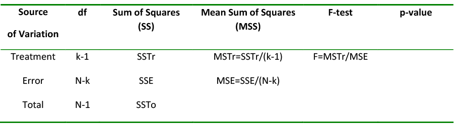
Table 1. One-way ANOVA table.
The sum of squares for the ANOVA table has the relationship of SSTo = SSTr + SSE where:
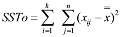
Total variation (SSTo) = explained variation (SSTr) + unexplained variation (SSE)
The degrees of freedom also have a similar relationship: df(SSTo) = df(SSTr) + df(SSE)
The Mean Sum of Squares for the treatment and error are found by dividing the Sums of Squares by the degrees of freedom for each. While the Sums of Squares are additive, the Mean Sums of Squares are not. The F-statistic is then found by dividing the Mean Sum of Squares for the treatment (MSTr) by the Mean Sum of Squares for the error(MSE). The MSTr is the SB2 and the MSE is the SW2.
F = SB2/ Sw2 = MSTr/MSE
Example 1
An environmentalist wanted to determine if the mean acidity of rain differed among Alaska, Florida, and Texas. He randomly selected six rain dates at each site obtained the following data:
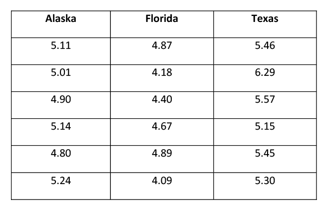
Table 2. Data for Alaska, Florida, and Texas.
H0: μA = μF = μT H1: at least one of the means is different
|
State |
Sample size |
Sample total |
Sample mean |
Sample variance |
|
Alaska |
n1 = 6 |
30.2 |
5.033 |
0.0265 |
|
Florida |
n2 = 6 |
27.1 |
4.517 |
0.1193 |
|
Texas |
n3 = 6 |
33.22 |
5.537 |
0.1575 |
Table 3. Summary Table.
Notice that there are differences among the sample means. Are the differences small enough to be explained solely by sampling variability? Or are they of sufficient magnitude so that a more reasonable explanation is that the μ’s are not all equal? The conclusion depends on how much variation among the sample means (based on their deviations from the grand mean) compares to the variation within the three samples.
The grand mean is equal to the sum of all observations divided by the total sample size:
 = grand total/N = 90.52/18 = 5.0289
SSTo = (5.11-5.0289)2 + (5.01-5.0289)2 +…+(5.24-5.0289)2
+ (4.87-5.0289)2 + (4.18-5.0289)2 +…+(4.09-5.0289)2
+ (5.46-5.0289)2 + (6.29-5.0289)2 +…+(5.30-5.0289)2 = 4.6384
SSTr = 6(5.033-5.0289)2 + 6(4.517-5.0289)2 + 6(5.537-5.0289)2 = 3.1214
SSE = SSTo – SSTr = 4.6384 – 3.1214 = 1.5170
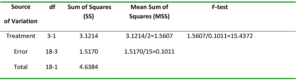
Table 4. One-way ANOVA Table.
This test is based on df1 = k – 1 = 2 and df2 = N – k = 15. For α = 0.05, the F critical value is 3.68. Since the observed F = 15.4372 is greater than the F critical value of 3.68, we reject the null hypothesis. There is enough evidence to state that at least one of the means is different.
Software Solutions
Minitab


One-way ANOVA: pH vs. State
|
Source |
DF |
SS |
MS |
F |
P |
|
State |
2 |
3.121 |
1.561 |
15.43 |
0.000 |
|
Error |
15 |
1.517 |
0.101 |
||
|
Total |
17 4.638 |
||||
|
S = 0.3180 R-Sq = 67.29% R-Sq(adj) = 62.93% |
|||||
|
Individual 95% CIs For Mean Based on Pooled StDev |
||||||||
|
Level |
N |
Mean |
StDev |
—-+———+———+———+—– |
||||
|
Alaska |
6 |
5.0333 |
0.1629 |
(——*——) |
||||
|
Florida |
6 |
4.5167 |
0.3455 |
(——*——) |
||||
|
Texas |
6 |
5.5367 |
0.3969 |
(——*——) |
||||
|
—-+———+———+———+—– |
||||||||
|
4.40 |
4.80 |
5.20 |
5.60 |
|||||
|
Pooled StDev = 0.3180 |
||||||||
The p-value (0.000) is less than the level of significance (0.05) so we will reject the null hypothesis.
Excel

 ANOVA: Single Factor
|
SUMMARY |
||||
|
Groups |
Count |
Sum |
Average |
Variance |
|
Column 1 |
6 |
30.2 |
5.033333 |
0.026547 |
|
Column 2 |
6 |
27.1 |
4.516667 |
0.119347 |
|
Column 3 |
6 |
33.22 |
5.536667 |
0.157507 |
|
ANOVA |
||||||
|
Source of Variation |
SS |
df |
MS |
F |
p-value |
F crit |
|
Between Groups |
3.121378 |
2 |
1.560689 |
15.43199 |
0.000229 |
3.68232 |
|
Within Groups |
1.517 |
15 |
0.101133 |
|||
|
Total |
4.638378 |
17 |
The p-value (0.000229) is less than alpha (0.05) so we reject the null hypothesis. There is enough evidence to support the claim that at least one of the means is different.
Once we have rejected the null hypothesis and found that at least one of the treatment means is different, the next step is to identify those differences. There are two approaches that can be used to answer this type of question: contrasts and multiple comparisons.
Contrasts can be used only when there are clear expectations BEFORE starting an experiment, and these are reflected in the experimental design. Contrasts are planned comparisons. For example, mule deer are treated with drug A, drug B, or a placebo to treat an infection. The three treatments are not symmetrical. The placebo is meant to provide a baseline against which the other drugs can be compared. Contrasts are more powerful than multiple comparisons because they are more specific. They are more able to pick up a significant difference. Contrasts are not always readily available in statistical software packages (when they are, you often need to assign the coefficients), or may be limited to comparing each sample to a control.
Multiple comparisons should be used when there are no justified expectations. They are aposteriori, pair-wise tests of significance. For example, we compare the gas mileage for six brands of all-terrain vehicles. We have no prior knowledge to expect any vehicle to perform differently from the rest. Pair-wise comparisons should be performed here, but only if an ANOVA test on all six vehicles rejected the null hypothesis first.
It is NOT appropriate to use a contrast test when suggested comparisons appear only after the data have been collected. We are going to focus on multiple comparisons instead of planned contrasts.
Multiple Comparisons
When the null hypothesis is rejected by the F-test, we believe that there are significant differences among the k population means. So, which ones are different? Multiple comparison method is the way to identify which of the means are different while controlling the experiment-wise error (the accumulated risk associated with a family of comparisons). There are many multiple comparison methods available.
In The Least Significant Difference Test, each individual hypothesis is tested with the student t-statistic. When the Type I error probability is set at some value and the variance s2 has v degrees of freedom, the null hypothesis is rejected for any observed value such that |to|>tα/2, v. It is an abbreviated version of conducting all possible pair-wise t-tests. This method has weak experiment-wise error rate. Fisher’s Protected LSD is somewhat better at controlling this problem.
Bonferroni inequality is a conservative alternative when software is not available. When conducting n comparisons, αe≤ n αc therefore αc = αe/n. In other words, divide the experiment-wise level of significance by the number of multiple comparisons to get the comparison-wise level of significance. The Bonferroni procedure is based on computing confidence intervals for the differences between each possible pair of μ’s. The critical value for the confidence intervals comes from a table with (N – k) degrees of freedom and k(k – 1)/2 number of intervals. If a particular interval does not contain zero, the two means are declared to be significantly different from one another. An interval that contains zero indicates that the two means are NOT significantly different.
Dunnett’s procedure was created for studies where one of the treatments acts as a control treatment for some or all of the remaining treatments. It is primarily used if the interest of the study is determining whether the mean responses for the treatments differ from that of the control. Like Bonferroni, confidence intervals are created to estimate the difference between two treatment means with a specific table of critical values used to control the experiment-wise error rate. The standard error of the difference is  .
.
Scheffe’s test is also a conservative method for all possible simultaneous comparisons suggested by the data. This test equates the F statistic of ANOVA with the t-test statistic. Since t2 = F then t = √F, we can substitute √F(αe, v1, v2) for t(αe, v2) for Scheffe’s statistic.
Tukey’s test provides a strong sense of experiment-wise error rate for all pair-wise comparison of treatment means. This test is also known as the Honestly Significant Difference. This test orders the treatments from smallest to largest and uses the studentized range statistic
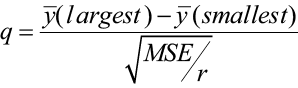
The absolute difference of the two means is used because the location of the two means in the calculated difference is arbitrary, with the sign of the difference depending on which mean is used first. For unequal replications, the Tukey-Kramer approximation is used instead.
Student-Newman-Keuls (SNK) test is a multiple range test based on the studentized range statistic like Tukey’s. The critical value is based on a particular pair of means being tested within the entire set of ordered means. Two or more ranges among means are used for test criteria. While it is similar to Tukey’s in terms of a test statistic, it has weak experiment-wise error rates.
Bonferroni, Dunnett’s, and Scheffe’s tests are the most conservative, meaning that the difference between the two means must be greater before concluding a significant difference. The LSD and SNK tests are the least conservative. Tukey’s test is in the middle. Robert Kuehl, author of Design of Experiments: Statistical Principles of Research Design and Analysis (2000), states that the Tukey method provides the best protection against decision errors, along with a strong inference about magnitude and direction of differences.
Let’s go back to our question on mean rain acidity in Alaska, Florida, and Texas. The null and alternative hypotheses were as follows:
|
H0: μA = μF = μT |
H1: at least one of the means is different |
The p-value for the F-test was 0.000229, which is less than our 5% level of significance. We rejected the null hypothesis and had enough evidence to support the claim that at least one of the means was significantly different from another. We will use Bonferroni and Tukey’s methods for multiple comparisons in order to determine which mean(s) is different.
Bonferroni Multiple Comparison Method
A Bonferroni confidence interval is computed for each pair-wise comparison. For k populations, there will be k(k-1)/2 multiple comparisons. The confidence interval takes the form of:
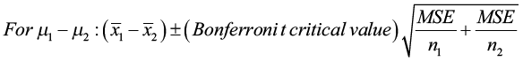

Where MSE is from the analysis of variance table and the Bonferroni t critical value comes from the Bonferroni Table given below. The Bonferroni t critical value, instead of the student t critical value, combined with the use of the MSE is used to achieve a simultaneous confidence level of at least 95% for all intervals computed. The two means are judged to be significantly different if the corresponding interval does not include zero.
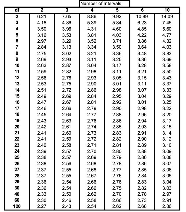
Table 5. Bonferroni t-critical values.
For this problem, k = 3 so there are k(k – 1)/2= 3(3 – 1)/2 = 3 multiple comparisons. The degrees of freedom are equal to N – k = 18 – 3 = 15. The Bonferroni critical value is 2.69.


The first confidence interval contains all positive values. This tells you that there is a significant difference between the two means and that the mean rain pH for Alaska is significantly greater than the mean rain pH for Florida.
The second confidence interval contains all negative values. This tells you that there is a significant difference between the two means and that the mean rain pH of Alaska is significantly lower than the mean rain pH of Texas.
The third confidence interval also contains all negative values. This tells you that there is a significant difference between the two means and that the mean rain pH of Florida is significantly lower than the mean rain pH of Texas.
All three states have significantly different levels of rain pH. Texas has the highest rain pH, then Alaska followed by Florida, which has the lowest mean rain pH level. You can use the confidence intervals to estimate the mean difference between the states. For example, the average rain pH in Texas ranges from 0.5262 to 1.5138 higher than the average rain pH in Florida.
Now let’s use the Tukey method for multiple comparisons. We are going to let software compute the values for us. Excel doesn’t do multiple comparisons so we are going to rely on Minitab output.

One-way ANOVA: pH vs. state
|
Source |
DF |
SS |
MS |
F |
P |
|
state |
2 |
3.121 |
1.561 |
15.4 |
0.000 |
|
Error |
15 |
1.517 |
0.101 |
||
|
Total |
17 |
4.638 |
|||
|
S = 0.3180 |
R-Sq = 67.29% |
R-Sq(adj) = 62.93% |
|||
We have seen this part of the output before. We now want to focus on the Grouping Information Using Tukey Method. All three states have different letters indicating that the mean rain pH for each state is significantly different. They are also listed from highest to lowest. It is easy to see that Texas has the highest mean rain pH while Florida has the lowest.
Grouping Information Using Tukey Method
|
state |
N |
Mean |
Grouping |
|
Texas |
6 |
5.5367 |
A |
|
Alaska |
6 |
5.0333 |
B |
|
Florida |
6 |
4.516 |
C |
|
Means that do not share a letter are significantly different. |
|||
This next set of confidence intervals is similar to the Bonferroni confidence intervals. They estimate the difference of each pair of means. The individual confidence interval level is set at 97.97% instead of 95% thus controlling the experiment-wise error rate.
|
Tukey 95% Simultaneous Confidence Intervals |
|
All Pairwise Comparisons among Levels of state |
|
Individual confidence level = 97.97% |
|
state = Alaska subtracted from: |
|||||||
|
state |
Lower |
Center |
Upper |
———+———+———+———+ |
|||
|
Florida |
-0.9931 |
-0.5167 |
-0.0402 |
(—–*—-) |
|||
|
Texas |
0.0269 |
0.5033 |
0.9798 |
(—–*—–) |
|||
|
———+———+———+———+ |
|||||||
|
-0.80 |
0.00 |
0.80 |
1.60 |
||||
|
state = Florida subtracted from: |
|||||||
|
state |
Lower |
Center |
Upper |
———+———+———+———+ |
|||
|
Texas |
0.5435 |
1.0200 |
1.4965 |
(—–*—–) |
|||
|
———+———+———+———+ |
|||||||
|
-0.80 |
0.00 |
0.80 |
1.60 |
||||
The first pairing is Florida – Alaska, which results in an interval of (-0.9931, -0.0402). The interval has all negative values indicating that Florida is significantly lower than Alaska. The second pairing is Texas – Alaska, which results in an interval of (0.0269, 0.9798). The interval has all positive values indicating that Texas is greater than Alaska. The third pairing is Texas – Florida, which results in an interval from (0.5435, 1.4965). All positive values indicate that Texas is greater than Florida.
The intervals are similar to the Bonferroni intervals with differences in width due to methods used. In both cases, the same conclusions are reached.
When we use one-way ANOVA and conclude that the differences among the means are significant, we can’t be absolutely sure that the given factor is responsible for the differences. It is possible that the variation of some other unknown factor is responsible. One way to reduce the effect of extraneous factors is to design an experiment so that it has a completely randomized design. This means that each element has an equal probability of receiving any treatment or belonging to any different group. In general good results require that the experiment be carefully designed and executed.
Additional example:
Candela Citations
- Natural Resources Biometrics. Authored by: Diane Kiernan. Located at: https://textbooks.opensuny.org/natural-resources-biometrics/. Project: Open SUNY Textbooks. License: CC BY-NC-SA: Attribution-NonCommercial-ShareAlike