Up to this point, we have discussed inferences regarding a single population parameter (e.g., μ, p, σ2). We have used sample data to construct confidence intervals to estimate the population mean or proportion and to test hypotheses about the population mean and proportion. In both of these chapters, all the examples involved the use of one sample to form an inference about one population. Frequently, we need to compare two sets of data, and make inferences about two populations. This chapter deals with inferences about two means, proportions, or variances. For example:
- You are studying turkey habitat and want to see if the mean number of brood hens is different in New York compared to Pennsylvania.
- You want to determine if the treatment used in Skaneateles Lake has reduced the number of milfoil plants over the last three years.
- Is the proportion of people who support alternative energy in California greater compared to New York?
- Is the variability in application different between two mist blowers?
These questions can be answered by comparing the differences of:
- Mean number of hens in NY to the mean number of hens in PA.
- Number of plants in 2007 to the number of plants in 2010.
- Proportion of people in CA to the proportion of people in NY.
- Variances between the mist blowers.
This chapter is comprised of five sections. The first and second sections examine inferences about two means with two independent samples. The third section examines inferences about means with two dependent samples, the fourth section examines inferences about two proportions, and the fifth section examines inferences between two variances.
Section 1
Inferences about Two Means with Independent Samples (Assuming Unequal Variances)
Using independent samples means that there is no relationship between the groups. The values in one sample have no association with the values in the other sample. For example, we want to see if the mean life span for hummingbirds in South Carolina is different from the mean life span in North Carolina. These populations are not related, and the samples are independent. We look at the difference of the independent means.
In Chapter 3, we did a one-sample t-test where we compared the sample mean ( ) to the hypothesized mean (μ). We expect that
  would be close to μ. We use the sample mean, the sample standard deviation, and the sample size for the one-sample test.
With a two-sample t-test, we compare the population means to each other and again look at the difference. We expect that  would be close to μ1 – μ2. The test statistic will use both sample means, sample standard deviations, and sample sizes for the test.
- For a one-sample t-test we used
 as a measure of the standard deviation (the standard error).
 - We can rewrite
 →
→ .
. - The numerator of the test statistic will be

- This has a standard deviation of
 .
.
A two-sample t-test follows the same four steps we saw in Chapter 3.
- Write the null and alternative hypotheses.
- State the level of significance and find the critical value. The critical value, from the student’s t-distribution, has the lesser of n1-1 and n2 -1 degrees of freedom.
- Compute the test statistic.
- Compare the test statistic to the critical value and state a conclusion.
The assumptions we saw in Chapter 3 still must be met. Both samples come from independent random samples. The populations must be normally distributed, or both have large enough sample sizes (n1 and n2 ≥ 30). We will also use the same three pairs of null and alternative hypotheses.
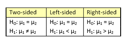
Table 1. Null and alternative hypotheses.
Rewriting the null hypothesis of μ1 = μ2 to μ1 – μ2 = 0, simplifies the numerator. The test statistic is Welch’s approximation (Satterthwaite Adjustment) under the assumption that the independent population variances are not equal.

This test statistic follows the student’s t-distribution with the degrees of freedom adjusted by

A simpler alternative to determining degrees of freedom when working a problem long-hand is to use the lesser of n1-1 or n2-1 as the degrees of freedom. This method results in a smaller value for degrees of freedom and therefore a larger critical value. This makes the test more conservative, requiring more evidence to reject the null hypothesis.
Example 1
A forester is studying the number of cavity trees in old growth stands in Adirondack Park in northern New York. He wants to know if there is a significant difference between the mean number of cavity trees in the Adirondack Park and the old growth stands in the Monongahela National Forest. He collects two independent random samples from each forest. Use a 5% level of significance to test this claim.
|
Adirondack Park |
Monongahela Forest |
|
n1 = 51 stands |
n2 = 56 stands |
|
|
|
|
s1 = 9.4 |
s2 = 10.7 |


1) H0: μ1 = μ2 or μ1 – μ2 = 0 There is no difference between the two population means.
H1: μ1 ≠ μ2 There is a difference between the two population means.
2) The level of significance is 5%. This is a two-sided test so alpha is split into two sides. Computing degrees of freedom using the equation above gives 105 degrees of freedom.

The critical value ( ), based on 100 degrees of freedom (closest value in the t-table), is ±1.984. Using 50 degrees of freedom, the critical value is ±2.009.
3) The test statistic is


4) The test statistic falls in the rejection zone.
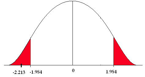
Figure 1. A comparison of the critical values and test statistic.
We reject the null hypothesis. We have enough evidence to support the claim that there is a difference in the mean number of cavity trees between the Adirondack Park and the Monongahela National Forest.
Construct and Interpret a Confidence Interval about the Difference of Two Independent Means
A hypothesis test will answer the question about the difference of the means. BUT, we can answer the same question by constructing a confidence interval about the difference of the means. This process is just like the confidence intervals from Chapter 2.
- Find the critical value.
- Compute the margin of error.
- Point estimate ± margin of error.
Because we are working with two samples, we must modify the components of the confidence interval to incorporate the information from the two populations.
- The point estimate is
 .
. - The standard error comes from the test statistic

- The critical value
 comes from the student’s t-table.
The confidence interval takes the form of the point estimate plus or minus the standard error of the differences.
 ±
± 

We will use the same three steps to construct a confidence interval about the difference of the means.
- critical value

- E =


 ± E
± E
Example 1a
Let’s look at the mean number of cavity trees in old growth stands again. The forester wants to know if there is a difference between the mean number of cavity trees in old growth stands in the Adirondack forests and in the Monongahela Forest. We can answer this question by constructing a confidence interval about the difference of the means.
1)  = 2.009
2) E = 
 = 2.009
  =3.904
3)  ± 3.904
The 95% confidence interval for the difference of the means is (-8.204, -0.396).
We can be 95% confident that this interval contains the mean difference in number of cavity trees between the two locations. BUT, this doesn’t answer the question the forester asked. Is there a difference in the mean number of cavity trees between the Adirondack and Monongahela forests? To answer this, we must look at the confidence interval interpretations.
Confidence Interval Interpretations
- If the confidence interval contains all positive values, we find a significant difference between the groups, AND we can conclude that the mean of the first group is significantly greater than the mean of the second group.
- If the confidence interval contains all negative values, we find a significant difference between the groups, AND we can conclude that the mean of the first group is significantly less than the mean of the second group.
- If the confidence interval contains zero (it goes from negative to positive values), we find NO significant difference between the groups.
In this problem, the confidence interval is (-8.204, -0.396). We have all negative values, so we can conclude that there is a significant difference in the mean number of cavity trees AND that the mean number of cavity trees in the Adirondack forests is significantly less than the mean number of cavity trees in the Monongahela Forest. The confidence interval gives an estimate of the mean difference in number of cavity trees between the two forests. There are, on average, 0.396 to 8.204 fewer cavity trees in the Adirondack Park than the Monongahela Forest.
P-value Approach
We can also use the p-value approach to answer the question. Remember, the p-value is the area under the normal curve associated with the test statistic. This example is a two-sided test (H1: μ1 ≠ μ2 ) so the p-value, when computed by hand, will be multiplied by two.
The test statistic equals -2.213, so the p-value is two times the area to the left of -2.213. We can only estimate the p-value using the student’s t-table. Using the lesser of n1– 1 or n2– 1 as the degrees of freedom, we have 50 degrees of freedom. Go across the 50 row in the student’s t-table until you find the absolute value of the test statistic. In this case, 2.213 falls between 2.109 and 2.403. Going up to the top of each of those columns gives you the estimate of the p-value (between 0.02 and 0.01).
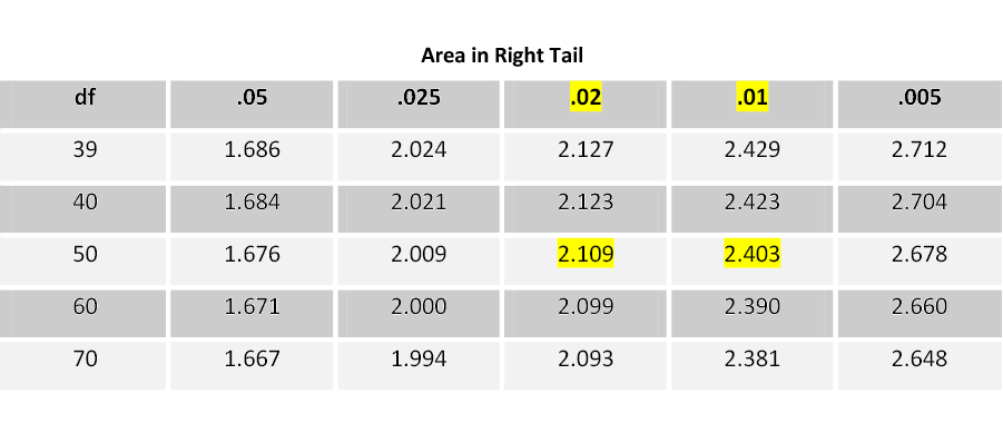
Table 2. Student t-Distribution
The p-value is 2x(0.01 – 0.02) = (0.02 < p < 0.04). The p-value is greater than 0.02 but less than 0.04. This is less than the level of significance (0.05), so we reject the null hypothesis. There is enough evidence to support the claim that there is a significant difference in the mean number of cavity trees between the areas.
Example 2
Researchers are studying the relationship between logging activities in the northern forests and amphibian habitats. They were comparing moisture levels between old-growth and post-harvest habitats. The researchers believe that post-harvest habitat has a lower moisture level. They collected data on moisture levels from two independent random samples. Test their claim using a 5% level of significance.
|
Old Growth |
Post Harvest |
|
n1 = 26 |
n2 = 31 |
|
|
|
|
s1 = 0.12 g/cm3 |
s2 = 0.17 g/cm3 |


H0: μ1 = μ2 or μ1 – μ2 = 0. There is no difference between the two population means.
H1: μ1 > μ2. Mean moisture level in old growth forests is greater than post-harvest levels.
We will use the critical value based on the lesser of n1– 1 or n2– 1 degrees of freedom. In this problem, there are 25 degrees of freedom and the critical value is 1.708. Now compute the test statistic.

The test statistic does not fall in the rejection zone. We fail to reject the null hypothesis. There is not enough evidence to support the claim that the moisture level is significantly lower in the post-harvest habitat.
Now answer this question by constructing a 90% confidence interval about the difference of the means.
1)  = 1.708
2) E = 

3)  ± E (0.62-0.56) ±0.0658
The 90% confidence interval for the difference of the means is (-0.0058, 0.1258). The values in the confidence interval run from negative to positive indicating that there is no significant different in the mean moisture levels between old growth and post-harvest stands.
Software Solutions
Minitab


|
Two-Sample T-Test and CI: old, post |
||||
|
Two-sample T for old vs. post |
||||
|
N |
Mean |
StDev |
SE Mean |
|
|
old |
26 |
0.620 |
0.121 |
0.024 |
|
post |
31 |
0.559 |
0.172 |
0.031 |
|
Difference = mu (old) – mu (post) |
||||
|
Estimate for difference: 0.0603 |
||||
|
95% lower bound for difference: -0.0049 |
||||
|
T-Test of difference = 0 (vs >): T-Value = 1.55 p-Value = 0.064 DF = 53 |
||||
The p-value (0.064) is greater than the level of confidence so we fail to reject the null hypothesis.
Additional example: www.youtube.com/watch?v=7pIb-GVixFo.
Excel


|
t-Test: Two-Sample Assuming Unequal Variances |
||
|
Variable 1 |
Variable 2 |
|
|
Mean |
0.619615 |
0.559355 |
|
Variance |
0.014708 |
0.02948 |
|
Observations |
26 |
31 |
|
Hypothesized Mean Difference |
0 |
|
|
df |
54 |
|
|
t Stat |
1.557361 |
|
|
P(T<=t) one-tail |
0.063809 |
|
|
t Critical one-tail |
1.673565 |
|
|
P(T<=t) two-tail |
0.127617 |
|
|
t Critical two-tail |
2.004879 |
|
The one-tail p-value (0.063809) is greater than the level of significance, therefore, we fail to reject the null hypothesis.
Section 2
Pooled Two-sampled t-test (Assuming Equal Variances)
In the previous section, we made the assumption of unequal variances between our two populations. Welch’s t-test statistic does not assume that the population variances are equal and can be used whether the population variances are equal or not. The test that assumes equal population variances is referred to as the pooled t-test. Pooling refers to finding a weighted average of the two independent sample variances.
The pooled test statistic uses a weighted average of the two sample variances.

If n1= n2, then S2p = (1/2)s21 + (1/2)s22, the average of the two sample variances. But whenever n1≠n2, the s2 based on the larger sample size will receive more weight than the other s2.
The advantage of this test statistic is that it exactly follows the student’s t-distribution with n1+ n2– 2 degrees of freedom.

The hypothesis test procedure will follow the same steps as the previous section.
It may be difficult to verify that two population variances might be equal based on sample data. The F-test is commonly used to test variances but is not robust. Small departures from normality greatly impact the outcome making the results of the F-test unreliable. It can be difficult to decide if a significant outcome from an F-test is due to the differences in variances or non-normality. Because of this, many researchers rely on Welch’s t when comparing two means.
Example 3
Growth of pine seedlings in two different substrates was measured. We want to know if growth was better in substrate 2. Growth (in cm/yr) was measured and included in the table below. α = 0.05
|
Substrate 1 |
Substrate 2 |
|
3.2 |
4.5 |
|
4.5 |
6.2 |
|
3.8 |
5.8 |
|
4.0 |
6.0 |
|
3.7 |
7.1 |
|
3.2 |
6.8 |
|
4.1 |
7.2 |
H0: μ1 = μ2
H1: μ1 < μ2


This is a one-sided test with n1 + n2 – 2 = 12 degrees of freedom. The critical value is -1.782. The test statistic is less than the critical value so we will reject the null hypothesis.
There is enough evidence to support the claim that the mean growth is less in substrate 1. Growth in substrate 2 is greater.
The confidence interval approach also uses the pooled variance and takes the form:

using n1 + n2 – 2 degrees of freedom. So let’s answer the same question with a 90% confidence interval.

All negative values tell you that there is a significant difference between the mean growth for the two substrates and that the growth in substrate 1 is significantly lower than the growth in substrate 2 with reduction in growth ranging from 1.734 to 3.146 cm/yr.
Software Solutions
Minitab


Two-Sample T-Test and CI: Substrate1, Substrate2
|
Two-sample T for Substrate1 vs. Substrate2 |
||||
|
N |
Mean |
StDev |
SE Mean |
|
|
Substrate1 |
7 |
3.786 |
0.474 |
0.18 |
|
Substrate2 |
7 |
6.229 |
0.936 |
0.35 |
|
Difference = mu (Substrate1) – mu (Substrate2) |
||||
|
Estimate for difference: -2.443 |
||||
|
95% upper bound for difference: -1.736 |
||||
|
T-Test of difference = 0 (vs <): T-Value = -6.16 p-value = 0.000 DF = 12 |
||||
|
Both use Pooled StDev = 0.7418 |
||||
The p-value (0.000) is less than the level of significance (0.05). We will reject the null hypothesis.
Excel

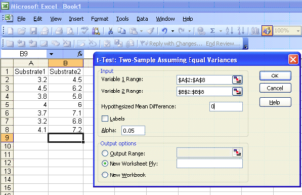
|
t-Test: Two-Sample Assuming Equal Variances |
||
|
Variable 1 |
Variable 2 |
|
|
Mean |
3.785714 |
6.228571 |
|
Variance |
0.224762 |
0.875714 |
|
Observations |
7 |
7 |
|
Pooled Variance |
0.550238 |
|
|
Hypothesized Mean Difference |
0 |
|
|
df |
12 |
|
|
t Stat |
-6.16108 |
|
|
P(T<=t) one-tail |
2.43E-05 |
|
|
t Critical one-tail |
1.782288 |
|
|
P(T<=t) two-tail |
4.86E-05 |
|
|
t Critical two-tail |
2.178813 |
|
This is a one-sided test (greater than) so use the P(T<=t) one-tail value 2.43E-05. The p-value (0.0000243) is less than the level of significance (0.05). We will reject the null hypothesis.
Section 3
Inferences about Two Means with Dependent Samples—Matched Pairs
Dependent samples occur when there is a relationship between the samples. The data consists of matched pairs from random samples. A sampling method is dependent when the values selected for one sample are used to determine the values in the second sample. Before and after measurements on a population, such as people, lakes, or animals are an example of dependent samples. The objects in your sample are measured twice; measurements are taken at a certain point in time, and then re-taken at a later date. Dependency also occurs when the objects are related, such as eyes or tires on a car. Pairing isn’t a problem; it’s an opportunity to use the information that occurs with both measurements.
Before you begin your work, you must decide if your samples are dependent. If they are, you can take advantage of this fact. You can use this matching to better answer your research questions. Pairing data reduces measurement variability, which increases the accuracy of our statistical conclusions.
We use the difference (the subtraction) of the pairs of data in our analysis. For each pair, we subtract the values:
- d1 = before1 – after 1
- d2 = before 2 – after 2
- d3 = before 3 – after 3
- …
We are creating a new random variable d (differences), and it is important to keep the sign, whether positive or negative. We can compute d̄, the sample mean of the differences, and sd, the sample standard deviation of the differences as follows:


Just as we used the sample mean and the sample standard deviation in a one-sample t-test, we will use the sample mean and sample standard deviation of the differences to test for matched pairs. The assumption of normality must still be verified. The differences must be normally distributed or the sample size must be large enough (n ≥ 30).
We can do a hypothesis test using matched pairs data following the same methods we used in the previous chapter.
- Write the null and alternative hypotheses.
- State the level of significance and find the critical value.
- Compute a test statistic.
- Compare the test statistic to the critical value and state a conclusion.
Since we are using the differences between the pairs of data, we identify this in our null and alternative hypotheses: H0: μd = 0. The mean of the differences is equal to zero; there is no difference in “before and after” values.
We’ll use the same three pairs of null and alternative hypotheses we used in the previous chapter.

Table 3. Null and alternative hypotheses.
The critical value comes from the student’s t-distribution table with n – 1 degrees of freedom, where n = number of matched pairs. The test statistic follows the student’s t-distribution

The conclusion must always answer the question you are asking in the alternative hypothesis.
- Reject the H0. There is enough evidence to support the alternative claim.
- Fail to reject the H0. There is not enough evidence to support the alternative claim.
Example 4
An environmental biologist wants to know if the water clarity in Owasco Lake is improving. Using a Secchi disk, she takes measurements in specific locations at specific dates during the course of the year. She then repeats the measurements in the same locations and on the same dates five years later. She obtains the following results:
|
Date |
Initial Depth |
5-year Depth |
Difference |
|
5/11 |
38 |
52 |
-14 |
|
6/7 |
58 |
60 |
-2 |
|
6/24 |
65 |
72 |
-7 |
|
7/8 |
74 |
72 |
2 |
|
7/27 |
56 |
54 |
2 |
|
8/31 |
36 |
48 |
-12 |
|
9/30 |
56 |
58 |
-2 |
|
10/12 |
52 |
60 |
-8 |
Using a 5% level of significance, test the biologist’s claim that water clarity is improving.
The data are paired by date with two measurements taken at each point five years apart. We will use the differences (right column) to see if there has been a significant improvement in water clarity. Using your calculator, Minitab, or Excel, compute the descriptive statistics on the differences to get the sample mean and the sample standard deviation of the differences.


1) The null and alternative hypotheses:
Ho: μd = 0 (The mean of the differences is equal to zero- no difference in water clarity over time.)
H1: μd < 0 (The water clarity is improving.)
We test “less than” because of how we computed the differences and the question we are asking.
In this case, we hope to see greater depth (better water clarity) at the five-year measurements. By calculating Initial – 5-year we hope to see negative values, values less than zero, indicating greater depth and clarity at the 5-year mark. Think of it like this:
Initial Depth < 5-year depth
This gives you the direction of the test!
2) The critical value tα.
The critical value comes from the student’s t-distribution table with n – 1 degrees of freedom. In this problem, we have eight pairs of data (n = 8) with 7 degrees of freedom. This is a one-sided test (less than), so alpha is all in the left tail. Go down the 0.05 column with 7 df to find the correct critical value (tα) of -1.895.
3) The test statistic  =
=  .
.
We subtract zero from d-bar because of our null hypothesis. Our null hypothesis is that the difference of the before and after values are statistically equal to zero. In other words, there has been no change in water clarity.
4) Compare the test statistic to the critical value and state a conclusion.
The test statistic (-2.38) is less than the critical value (-1.895). It falls in the rejection zone.

Figure 2. Comparison of the critical value and the test statistic.
We reject the null hypothesis. We have enough evidence to support the claim that the mean water clarity has improved.
P-value Approach
We can also use the p-value approach to answer the question. To estimate p-value using the student’s t-table, go across the row for 7 degrees of freedom until you find the two values that the absolute value of your test statistic falls between.
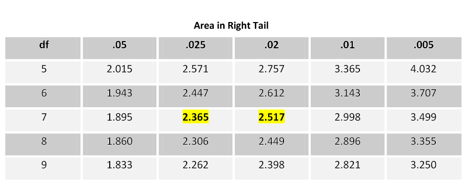
Table 4. Student t-Distribution.
The p-value for this test statistic is greater than 0.02 and just less than 0.025. Compare this to the level of significance (alpha). The Decision Rule says that if the p-value is less than α, reject the null hypothesis. In this case, the p-value estimate (0.02 – 0.025) is less than the level of significance (0.05). Reject the null hypothesis. We have enough evidence to support the claim that the mean water clarity has improved.
BUT, what if you used a 1% level of significance? In this case, the p-value is NOT less than the level of significance ((0.02 – 0.025)>0.01). We would fail to reject the null hypothesis. There is NOT enough evidence to support the claim that the water clarity has improved. It is important to set the level of significance at the start of your research and report the p-value. Another researcher may interpret your findings differently, based on your reported p-value and their own selected level of significance.
Construct and Interpret a Confidence Interval about the Differences of the Data for Matched Pairs
A hypothesis test for matched pairs data is very similar to a one-sample t-test. BUT, we can answer the same question by constructing a confidence interval about the mean of the differences. This process is just like the confidence intervals from Chapter 2.
- Find the critical value.
- Compute the margin of error.
- Point estimate ± margin of error.
For matched pairs data, the critical value comes from the student’s t-distribution with n – 1 degrees of freedom. The margin of error uses the sample standard deviation of the differences (sd) and the point estimate is d̄, the mean of the differences.
For a (1 – α)*100% confidence interval for the mean of the differences

- Where
 is used because confidence intervals are always two-sided.
Example 4a
Let’s look at the biologist studying water clarity in Owasco Lake again. She wants to test the claim that water clarity has improved. We can answer this question by constructing a confidence interval about the mean of the differences.
|
d̄ = -5.125 |
sd = 6.081 |
α = 0.05 |
n = 8 |
1) 
2)  =
= 
3) 
The 95% confidence interval about the mean of the differences is
(-10.21, -0.04)
(-10.21≤ μd ≤ -0.04)
We can be 95% confident that this interval contains the true mean of the differences in water clarity between the two time periods. BUT, this doesn’t directly answer the question about improved water clarity. To do this, we use the interpretations given below.
Confidence Interval Interpretations
- If the confidence interval contains all positive values, we find a significant difference between the groups, AND we can conclude that the mean of the first group is significantly greater than the mean of the second group.
- If the confidence interval contains all negative values, we find a significant difference between the groups, AND we can conclude that the mean of the first group is significantly less than the mean of the second group.
- If the confidence interval contains zero (it goes from negative to positive values), we find NO significant difference between the groups.
In this problem, the confidence interval is (-10.21, -0.04). We have all negative values, so we can conclude that there is a significant difference in the mean water clarity between the years AND…
- The mean water clarity for the initial time was significantly less than at the five-year re-measurement.
- Water clarity has improved during the five-year period. The confidence interval estimates the mean improvement.
Example 5
Biologists are studying elk migration in the western US and want to know if the four-lane interstate that was built ten years ago has disturbed elk migration to the winter feeding area. A random sample was gathered from nine wilderness districts in the winter feeding areas. These data were compared to a random sample collected from the same nine areas before the highway was built. Use a 1% level of significance to test this claim.
|
District |
1 |
2 |
3 |
4 |
5 |
6 |
7 |
8 |
9 |
|
Before |
11.6 |
18.7 |
15.9 |
20.6 |
10.1 |
17.4 |
7.2 |
12.2 |
11.7 |
|
After |
10.0 |
21.6 |
13.9 |
22.8 |
11.5 |
16.2 |
8.1 |
10.8 |
9.6 |
|
d |
1.6 |
-2.9 |
2.0 |
-2.2 |
-1.4 |
1.2 |
-0.9 |
1.4 |
2.1 |

H0: μd = 0
H1: μd ≠ 0
Determine the critical values: This is a two-sided question (alternative ≠) so the critical values are ±3.355.
Compute the test statistic:

Now compare the critical value to the test statistic and state a conclusion. The test statistic is NOT greater than 3.355 or less than -3.355 (it doesn’t fall in the rejection zones). We fail to reject the null hypothesis. There is not enough evidence to support the claim that the highway has interfered with the elk migration (no difference before or after the highway).
Now construct a 99% confidence interval and answer the question.
1)  = 3.355
2) 
3)  0.100±2.176
The 99% confidence interval about the difference of the means is: (-2.076, 2.276)
This confidence interval contains zero. The null hypothesis is that there is zero difference before and after the highway way was created. Therefore, we fail to reject the null hypothesis. There is not enough evidence to support the claim that the highway has interfered with the elk migration (no difference before or after the highway).
Software Solutions
Minitab


Paired T-Test and CI: Before, After
|
Paired T for Before – After |
||||
|
N |
Mean |
StDev |
SE Mean |
|
|
Before |
9 |
13.93 |
4.42 |
1.47 |
|
After |
9 |
13.83 |
5.32 |
1.77 |
|
Difference |
9 |
0.100 |
1.946 |
0.649 |
|
99% CI for mean difference: (-2.077, 2.277) |
||||
|
T-Test of mean difference = 0 (vs not = 0): T-Value = 0.15 p-value = 0.881 |
||||
Minitab gives the test statistic of 0.15 and the p-value of 0.881. It also gives a 99% confidence interval for the difference of the means (-2.077, 2.277). All results support failing to reject the null hypothesis.
Excel


|
t-Test: Paired Two Sample for Means |
||
|
Before |
After |
|
|
Mean |
13.93333 |
13.83333333 |
|
Variance |
19.565 |
28.3075 |
|
Observations |
9 |
9 |
|
Pearson Correlation |
0.936635 |
|
|
Hypothesized Mean Difference |
0 |
|
|
df |
8 |
|
|
t Stat |
0.15415 |
|
|
P(T<=t) one-tail |
0.440654 |
|
|
t Critical one-tail |
2.896459 |
|
|
P(T<=t) two-tail |
0.881309 |
|
|
t Critical two-tail |
3.355387 |
|
The test statistic is 0.15415. This is a two-sided question so we can use P(T<=t) two-tail = 0.881309. The p-value is NOT less than the 1% level of significance so we will fail to reject the null hypothesis.
Section 4
Inferences about Two Population Proportions
We can apply the same methods we just learned with means to our two-sample proportion problems. We have two populations with two samples and we want to compare the population proportions.
- Is the proportion of lakes in New York with invasive species different from the proportion of lakes in Michigan with invasive species?
- Is the proportion of construction companies using certified lumber greater in the northeast than in the southeast?
A test of two population proportions is very similar to a test of two means, except that the parameter of interest is now “p” instead of “µ”. With a one-sample proportion test, we used  as the point estimate of p. We expect that p̂ would be close to p. With a test of two proportions, we will have two p̂’s, and we expect that (p̂1 – p̂2) will be close to (p1 – p2). The test statistic accounts for both samples.
- With a one-sample proportion test, the test statistic is

and it has an approximate standard normal distribution.
- For a two-sample proportion test, we would expect the test statistic to be

HOWEVER, the null hypothesis will be that p1 = p2. Because the H0 is assumed to be true, the test assumes that p1 = p2. We can then assume that p1 = p2 equals p, a common population proportion. We must compute a pooled estimate of p (its unknown) using our sample data.

The test statistic then takes the form of

The hypothesis test follows the same steps that we have seen in previous sections:
- State the null and alternative hypotheses
- State the level of significance and determine the critical value
- Compute the test statistic
- Compare the critical value and the test statistic and state a conclusion
The assumptions that we set for a one-sample proportion test still hold true for both samples. Both must be random samples from normally distributed populations satisfying the following statements:
- n(p)(1 – p) ≥ 10
- Each sample size is no more than 5% of the population size.
We can again use the same three pairs of null and alternative hypotheses. Notice that we are working with population proportions so the parameter is p.

Table 5. Null and alternative hypotheses.
The critical value comes from the standard normal table and depends on the alternative hypothesis (is the question one- or two-sided?). As usual, you must state a conclusion. You must always answer the question that is asked in the alternative hypothesis.
Example 6
A researcher believes that a greater proportion of construction companies in the northeast are using certified lumber in home construction projects compared to companies in the southeast. She collected a random sample of 173 companies in the southeast and found that 86 used at least 30% certified lumber. She collected another random sample of 115 companies from the northeast and found that 68 used at least 30% certified lumber. Test the researcher’s claim that a greater proportion of companies in the northeast use at least 30% certified lumber compared to the southeast. α = 0.05.
| Southeast | Northeast |
| n1 = 173 | n2 = 115 |
| x1 = 86 | x2 = 68 |
Write the null and alternative hypotheses:
H0: p1 = p2 or p1 – p2 = 0
H1: p1 < p2
The critical value comes from the standard normal table. It is a one-sided test, so alpha is all in the left tail. The critical value is -1.645.
Compute the point estimates


Now compute p̄
 =
=
The test statistic is
 =
=  = -1.57.
Now compare the critical value to the test statistic and state a conclusion.
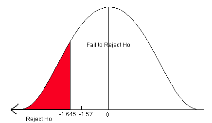
Figure 3. A comparison of the critical value and the test statistic.
We fail to reject the null hypothesis. There is not enough evidence to support the claim that a greater proportion of companies in the northeast use at least 30% certified lumber compared to companies in the southeast.
Using the P-Value Approach
We can also answer this question using the p-value approach. The p-value is the area associated with the test statistic. This is a left-tailed problem with a test statistic of -1.57 so the p-value is the area to the left of -1.57. Look up the area associated with the Z-score -1.57 in the standard normal table.
The p-value is 0.0582.
The hatched area (p-value) is greater than the 5% level of significance (red area). We fail to reject the null hypothesis. There is not enough statistical evidence to support the claim that a greater proportion of companies in the northeast use at least 30% certified lumber compared to companies in the southeast.
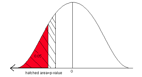
Figure 4. Comparison of p-value and the level of significance.
Construct and Interpret a Confidence Interval about the Difference of Two Proportions
Just like a two-sample t-test about the means, we can answer this question by constructing a confidence interval about the difference of the proportions. The point estimate is p̂1 – p̂2. The standard error is  and the critical value
  comes from the standard normal table.
The confidence interval takes the form of the point estimate ± the margin of error.
 ±
± 

We will use the same three steps to construct a confidence interval about the difference of the proportions. Notice the estimate of the standard error of the differences. We do not rely on the pooled estimate of p when constructing confidence intervals to estimate the difference in proportions. This is because we are not making any assumptions regarding the equality of p1 and p2, as we did in the hypothesis test.
1) critical value 
2) E = 

3)  ± E
± E
Let’s revisit Ex. 6 again, but this time we will construct a confidence interval about the difference between the two proportions.
Example 6a
The researcher claims that a greater proportion of companies in the northeast use at least 30% certified lumber compared to companies in the southeast. We can test this claim by constructing a 90% confidence interval about the difference of the proportions.
1) critical value  = 1.645
2) E = 
 =
=  = 0.098
3)  ± E = (0.497-0.591) ± 0.098
The 90% confidence interval about the difference of the proportions is (-0.192, 0.004).
BUT, this doesn’t answer the question the researcher asked. We must use one of the three interpretations seen in the previous section. In this problem, the confidence interval contains zero. Therefore we can conclude that there is no significant difference between the proportions of companies using certified lumber in the northeast and in the southeast.
Example 7
A hydrologist is studying the use of Best Management Plans (BMP) in managed forest stands to protect riparian zones. He collects information from 62 stands that had a management plan by a forester and finds that 47 stands had correctly implemented BMPs to protect the riparian zones. He collected information from 58 stands that had no management plan and found that 26 of them had correctly implemented BMPs for riparian zones. Do these data suggest that there is a significant difference in the proportion of stands with and without management plans that had correct BMPs for riparian zones? α = 0.05.
| Plan | No Plan |
| x1 = 47 | x2 = 26 |
| n1 = 62 | n2 = 58 |
Let’s answer this question both ways by first using a hypothesis test and then by constructing a confidence interval about the difference of the proportions.
H0: p1 = p2 or p1 – p2 = 0
H1: p1 ≠ p2
Critical value: ±1.96
Test statistic:

The test statistic is greater than 1.96 and falls in the rejection zone. There is enough evidence to support the claim that there is a significant difference in the proportion of correctly implemented BMPs with and without management plans.
Now compute the p-value and compare it to the level of significance. The p-value is two times the area under the curve to the right of 3.48. Look for the area (in the standard normal table) associated with a Z-score of 3.48. The area to the right of 3.48 is 1 – 0.9997 = 0.0003. The p-value is 2 x 0.0003 = 0.0006.
The p-value is less than 0.05. We will reject the null hypothesis and support the claim that the proportions are different.
Now, answer this question using a confidence interval.
1) critical value  = 1.96
2) E = 

3)  ± E (0.758,-0.448) ± 0.1666
The 95% confidence interval about the difference of the proportions is (0.143, 0.477). The confidence interval contains all positive values, telling you that there is a significant difference between the proportions AND the first group (BMPs used with management plans) is significantly greater than the second group (BMPs with no plans). This confidence interval estimates the difference in proportions. For this problem, we can say that correctly implemented BMPs with a plan occur in a greater proportion (14.3% to 44.7%) compared to those implemented without a management plan.
Software Solutions
Minitab


Test and CI for Two Proportions
|
Sample |
X |
N |
Sample p |
|
1 |
47 |
62 |
0.758065 |
|
2 |
26 |
58 |
0.448276 |
|
Difference = p (1) – p (2) |
|||
|
Estimate for difference: 0.309789 |
|||
|
95% CI for difference: (0.143223, 0.476355) |
|||
|
Test for difference = 0 (vs. not = 0): Z = 3.47 p-value = 0.001 |
|||
|
Fisher’s exact test: p-value = 0.001 |
|||
The p-value equals 0.001 which tells us to reject the null hypothesis. There is a significant difference in the proportion of correctly implemented BMPs with and without management plans. The confidence interval for the difference in proportions is also given (0.143223, 0.476355) which allows us to estimate the difference.
Excel
Excel does not analyze data from proportions.
Section 5
F-Test for Comparing Two Population Variances
One major application of a test for the equality of two population variances is for checking the validity of the equal variance assumption ( ) for a two-sample t-test. First we hypothesize two populations of measurements that are normally distributed. We label these populations as 1 and 2, respectively. We are interested in comparing the variance of population 1 (
 ) to the variance of population 2 (
 ).
).
When independent random samples have been drawn from the respective populations, the ratio

possesses a probability distribution in repeated sampling that is referred to as an F distribution and its properties are:
- Unlike Z and t, but like χ2, F can assume only positive values.
- The F distribution, unlike the Z and t distributions, but like the χ2 distribution, is non-symmetrical.
- There are many F distributions, and each one has a different shape. We specify a particular one by designating the degrees of freedom associated with
 and
and  . We denote these quantities by df1 and df2, respectively.
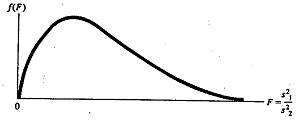
Figure 5. The F-distribution.
Note: A statistical test of the null hypothesis  utilizes the test statistic
  . It may require either upper tail or lower tail rejection region, depending on which sample variance is larger. To alleviate this situation, we are at liberty to designate the population with the larger sample variance as population 1 (i.e., used as the numerator of the ratio
  ). By this convention, the rejection region is only located in the upper tail of the F distribution.
Null hypothesis: H0: 
Alternative hypothesis:
- Ha:
 >
>  (one-tailed), reject H0 if the observed F > Fα
 - Ha:
 ≠
≠  (two-tailed), reject H0 if the observed F > Fα/2.
Test statistic:  assuming
  >
>  ,
,
where the F critical value in the rejection region is based on 2 degrees of freedom df1 = n1 – 1 (associated with numerator  ) and df2 = n2 – 1 (associated with denominator
  ).
).
Example 8
A forester wants to compare two different mist blowers for consistent application. She wants to use the mist blower with the smaller variance, which means more consistent application. She wants to test that the variance of Type A (0.087 gal.2) is significantly greater than the variance of Type B (0.073 gal.2) using α = 0.05.
| Type A | Type B |
| S21 = 0.087 | S22=0.073 |
| n1= 16 | n2 = 21 |
H0: 
H1:  >
> 
The critical value (df1 = 15 and df2 = 20) is 2.20.
The test statistic is:

The test statistic is not larger than the critical value (it does not fall in the rejection zone) so we fail to reject the null hypothesis. While the variance of Type B is mathematically smaller than the variance of Type A, it is not statistically smaller. There is not enough statistical evidence to support the claim that the variance of Type A is significantly greater than the variance of Type B. Both mist blowers will deliver the chemical with equal consistency.
Software Solutions
Minitab

 Test and CI for Two Variances
|
Method |
|||||
|
Null hypothesis |
Variance(1) / Variance(2) = 1 |
||||
|
Alternative hypothesis |
Variance(1) / Variance(2) > 1 |
||||
|
Significance level |
Alpha = 0.05 |
||||
|
Statistics |
|||||
|
Sample |
N |
StDev |
Variance |
||
|
1 |
16 |
0.295 |
0.087 |
||
|
2 |
21 |
0.270 |
0.073 |
||
|
Ratio of standard deviations = 1.092 |
|||||
|
Ratio of variances = 1.192 |
|||||
|
Tests |
|||||
|
Test |
|||||
|
Method |
DF1 |
DF2 |
Statistic |
p-value |
|
|
F Test (normal) |
15 |
20 |
1.19 |
0.351 |
|
Excel


F-Test Two-Sample for Variances
|
Type A |
Type B |
|
|
Mean |
11.07188 |
11.10595 |
|
Variance |
0.08699 |
0.073379 |
|
Observations |
16 |
21 |
|
df |
15 |
20 |
|
F |
1.185483 |
|
|
P(F<=f) one-tail |
0.355098 |
|
|
F Critical one-tail |
2.203274 |
Summary
Questions about the differences between two samples can be answered in several ways: hypothesis test, p-value approach, or confidence interval approach. In all cases, you must clearly state your question, the selected level of significance and the conclusion.
If you choose the hypothesis test approach, you need to compare the critical value to the test statistic. If the test statistic falls in the rejection zone set by the critical value, then you will reject the null hypothesis and support the alternative claim.
If you use the p-value approach, you must compute the test statistic and find the area associated with that value. For a two-sided test, the p-value is two times the area of the absolute value of the test statistic. For a one-sided test, the p-value is the area to the left or right of the test statistic. The decision rule states: If the p-value is less than α(level of significance), reject the null hypothesis and support the alternative claim.
The confidence interval approach constructs an interval about the difference of the means or proportions. If the interval contains zero, then you can conclude that there is no difference between the two groups. If the interval contains all positive values, you can conclude that group 1 is significantly greater than group 2. If the interval contains all negative numbers, you can conclude that group 2 is significantly greater than group 1.
In all approaches, a clear and concise conclusion is required. You MUST answer the question being asked by stating the results of your approach.
Candela Citations
- Natural Resources Biometrics. Authored by: Diane Kiernan. Located at: https://textbooks.opensuny.org/natural-resources-biometrics/. Project: Open SUNY Textbooks. License: CC BY-NC-SA: Attribution-NonCommercial-ShareAlike