Section 1
The previous two chapters introduced methods for organizing and summarizing sample data, and using sample statistics to estimate population parameters. This chapter introduces the next major topic of inferential statistics: hypothesis testing.
A hypothesis is a statement or claim about a property of a population.
The Fundamentals of Hypothesis Testing
When conducting scientific research, typically there is some known information, perhaps from some past work or from a long accepted idea. We want to test whether this claim is believable. This is the basic idea behind a hypothesis test:
- State what we think is true.
- Quantify how confident we are about our claim.
- Use sample statistics to make inferences about population parameters.
For example, past research tells us that the average life span for a hummingbird is about four years. You have been studying the hummingbirds in the southeastern United States and find a sample mean lifespan of 4.8 years. Should you reject the known or accepted information in favor of your results? How confident are you in your estimate? At what point would you say that there is enough evidence to reject the known information and support your alternative claim? How far from the known mean of four years can the sample mean be before we reject the idea that the average lifespan of a hummingbird is four years?
Hypothesis testing is a procedure, based on sample evidence and probability, used to test claims regarding a characteristic of a population.
A hypothesis is a claim or statement about a characteristic of a population of interest to us. A hypothesis test is a way for us to use our sample statistics to test a specific claim.
Example 1
The population mean weight is known to be 157 lb. We want to test the claim that the mean weight has increased.
Example 2
Two years ago, the proportion of infected plants was 37%. We believe that a treatment has helped, and we want to test the claim that there has been a reduction in the proportion of infected plants.
Components of a Formal Hypothesis Test
The null hypothesis is a statement about the value of a population parameter, such as the population mean (µ) or the population proportion (p). It contains the condition of equality and is denoted as H0 (H-naught).
H0 : µ = 157 or H0 : p = 0.37
The alternative hypothesis is the claim to be tested, the opposite of the null hypothesis. It contains the value of the parameter that we consider plausible and is denoted as H1 .
H1 : µ > 157 or H1 : p ≠ 0.37
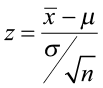
The test statistic is a value computed from the sample data that is used in making a decision about the rejection of the null hypothesis. The test statistic converts the sample mean (x̄) or sample proportion (p̂) to a Z- or t-score under the assumption that the null hypothesis is true. It is used to decide whether the difference between the sample statistic and the hypothesized claim is significant.
The p-value is the area under the curve to the left or right of the test statistic. It is compared to the level of significance (α).
The critical value is the value that defines the rejection zone (the test statistic values that would lead to rejection of the null hypothesis). It is defined by the level of significance.
The level of significance (α) is the probability that the test statistic will fall into the critical region when the null hypothesis is true. This level is set by the researcher.
The conclusion is the final decision of the hypothesis test. The conclusion must always be clearly stated, communicating the decision based on the components of the test. It is important to realize that we never prove or accept the null hypothesis. We are merely saying that the sample evidence is not strong enough to warrant the rejection of the null hypothesis. The conclusion is made up of two parts:
1) Reject or fail to reject the null hypothesis, and 2) there is or is not enough evidence to support the alternative claim.
Option 1) Reject the null hypothesis (H0). This means that you have enough statistical evidence to support the alternative claim (H1).
Option 2) Fail to reject the null hypothesis (H0). This means that you do NOT have enough evidence to support the alternative claim (H1).
Another way to think about hypothesis testing is to compare it to the US justice system. A defendant is innocent until proven guilty (Null hypothesis—innocent). The prosecuting attorney tries to prove that the defendant is guilty (Alternative hypothesis—guilty). There are two possible conclusions that the jury can reach. First, the defendant is guilty (Reject the null hypothesis). Second, the defendant is not guilty (Fail to reject the null hypothesis). This is NOT the same thing as saying the defendant is innocent! In the first case, the prosecutor had enough evidence to reject the null hypothesis (innocent) and support the alternative claim (guilty). In the second case, the prosecutor did NOT have enough evidence to reject the null hypothesis (innocent) and support the alternative claim of guilty.
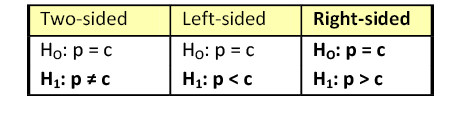
The Null and Alternative Hypotheses
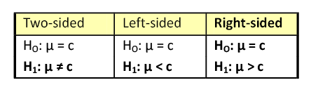
There are three different pairs of null and alternative hypotheses:
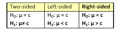
where c is some known value.
A Two-sided Test
This tests whether the population parameter is equal to, versus not equal to, some specific value.
Ho: μ = 12 vs. H1: μ ≠ 12
The critical region is divided equally into the two tails and the critical values are ± values that define the rejection zones.

Figure 1. The rejection zone for a two-sided hypothesis test.
Example 3
A forester studying diameter growth of red pine believes that the mean diameter growth will be different if a fertilization treatment is applied to the stand.
- Ho: μ = 1.2 in./ year
- H1: μ ≠ 1.2 in./ year
This is a two-sided question, as the forester doesn’t state whether population mean diameter growth will increase or decrease.
A Right-sided Test
This tests whether the population parameter is equal to, versus greater than, some specific value.
Ho: μ = 12 vs. H1: μ > 12
The critical region is in the right tail and the critical value is a positive value that defines the rejection zone.
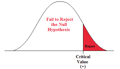
Figure 2. The rejection zone for a right-sided hypothesis test.
Example 4
A biologist believes that there has been an increase in the mean number of lakes infected with milfoil, an invasive species, since the last study five years ago.
- Ho: μ = 15 lakes
- H1: μ >15 lakes
This is a right-sided question, as the biologist believes that there has been an increase in population mean number of infected lakes.
A Left-sided Test
This tests whether the population parameter is equal to, versus less than, some specific value.
Ho: μ = 12 vs. H1: μ < 12
The critical region is in the left tail and the critical value is a negative value that defines the rejection zone.
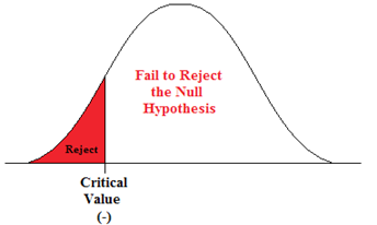
Figure 3. The rejection zone for a left-sided hypothesis test.
Example 5
A scientist’s research indicates that there has been a change in the proportion of people who support certain environmental policies. He wants to test the claim that there has been a reduction in the proportion of people who support these policies.
- Ho: p = 0.57
- H1: p < 0.57
This is a left-sided question, as the scientist believes that there has been a reduction in the true population proportion.
Statistically Significant
When the observed results (the sample statistics) are unlikely (a low probability) under the assumption that the null hypothesis is true, we say that the result is statistically significant, and we reject the null hypothesis. This result depends on the level of significance, the sample statistic, sample size, and whether it is a one- or two-sided alternative hypothesis.
Types of Errors
When testing, we arrive at a conclusion of rejecting the null hypothesis or failing to reject the null hypothesis. Such conclusions are sometimes correct and sometimes incorrect (even when we have followed all the correct procedures). We use incomplete sample data to reach a conclusion and there is always the possibility of reaching the wrong conclusion. There are four possible conclusions to reach from hypothesis testing. Of the four possible outcomes, two are correct and two are NOT correct.
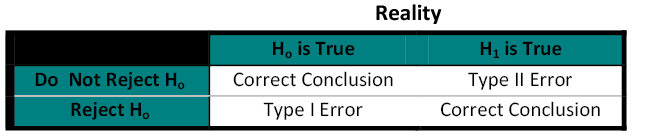
Table 1. Possible outcomes from a hypothesis test.
A Type I error is when we reject the null hypothesis when it is true. The symbol α (alpha) is used to represent Type I errors. This is the same alpha we use as the level of significance. By setting alpha as low as reasonably possible, we try to control the Type I error through the level of significance.
A Type II error is when we fail to reject the null hypothesis when it is false. The symbol β (beta) is used to represent Type II errors.
In general, Type I errors are considered more serious. One step in the hypothesis test procedure involves selecting the significance level (α), which is the probability of rejecting the null hypothesis when it is correct. So the researcher can select the level of significance that minimizes Type I errors. However, there is a mathematical relationship between α, β, and n (sample size).
- As α increases, β decreases
- As α decreases, β increases
- As sample size increases (n), both α and β decrease
The natural inclination is to select the smallest possible value for α, thinking to minimize the possibility of causing a Type I error. Unfortunately, this forces an increase in Type II errors. By making the rejection zone too small, you may fail to reject the null hypothesis, when, in fact, it is false. Typically, we select the best sample size and level of significance, automatically setting β.
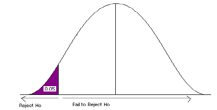
Figure 4. Type 1 error.
Power of the Test
A Type II error (β) is the probability of failing to reject a false null hypothesis. It follows that 1-β is the probability of rejecting a false null hypothesis. This probability is identified as the power of the test, and is often used to gauge the test’s effectiveness in recognizing that a null hypothesis is false.
The probability that at a fixed level α significance test will reject H0, when a particular alternative value of the parameter is true is called the power of the test.
Power is also directly linked to sample size. For example, suppose the null hypothesis is that the mean fish weight is 8.7 lb. Given sample data, a level of significance of 5%, and an alternative weight of 9.2 lb., we can compute the power of the test to reject μ = 8.7 lb. If we have a small sample size, the power will be low. However, increasing the sample size will increase the power of the test. Increasing the level of significance will also increase power. A 5% test of significance will have a greater chance of rejecting the null hypothesis than a 1% test because the strength of evidence required for the rejection is less. Decreasing the standard deviation has the same effect as increasing the sample size: there is more information about μ.
Section 2
Hypothesis Test about the Population Mean (μ) when the Population Standard Deviation (σ) is Known
We are going to examine two equivalent ways to perform a hypothesis test: the classical approach and the p-value approach. The classical approach is based on standard deviations. This method compares the test statistic (Z-score) to a critical value (Z-score) from the standard normal table. If the test statistic falls in the rejection zone, you reject the null hypothesis. The p-value approach is based on area under the normal curve. This method compares the area associated with the test statistic to alpha (α), the level of significance (which is also area under the normal curve). If the p-value is less than alpha, you would reject the null hypothesis.
As a past student poetically said: If the p-value is a wee value, Reject Ho
Both methods must have:
- Data from a random sample.
- Verification of the assumption of normality.
- A null and alternative hypothesis.
- A criterion that determines if we reject or fail to reject the null hypothesis.
- A conclusion that answers the question.
There are four steps required for a hypothesis test:
- State the null and alternative hypotheses.
- State the level of significance and the critical value.
- Compute the test statistic.
- State a conclusion.
The Classical Method for Testing a Claim about the Population Mean (μ) when the Population Standard Deviation (σ) is Known
Example 6
A Two-sided Test
A forester studying diameter growth of red pine believes that the mean diameter growth will be different from the known mean growth of 1.35 inches/year if a fertilization treatment is applied to the stand. He conducts his experiment, collects data from a sample of 32 plots, and gets a sample mean diameter growth of 1.6 in./year. The population standard deviation for this stand is known to be 0.46 in./year. Does he have enough evidence to support his claim?
Step 1) State the null and alternative hypotheses.
- Ho: μ = 1.35 in./year
- H1: μ ≠ 1.35 in./year
Step 2) State the level of significance and the critical value.
- We will choose a level of significance of 5% (α = 0.05).
- For a two-sided question, we need a two-sided critical value – Z α/2 and + Z α/2.
- The level of significance is divided by 2 (since we are only testing “not equal”). We must have two rejection zones that can deal with either a greater than or less than outcome (to the right (+) or to the left (-)).
- We need to find the Z-score associated with the area of 0.025. The red areas are equal to α/2 = 0.05/2 = 0.025 or 2.5% of the area under the normal curve.
- Go into the body of values and find the negative Z-score associated with the area 0.025.
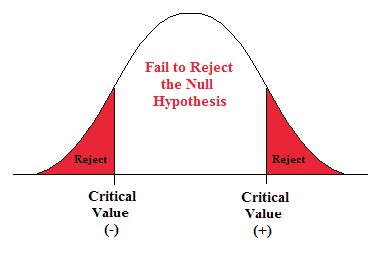
Figure 5. The rejection zone for a two-sided test.
- The negative critical value is -1.96. Since the curve is symmetric, we know that the positive critical value is 1.96.
- ±1.96 are the critical values. These values set up the rejection zone. If the test statistic falls within these red rejection zones, we reject the null hypothesis.
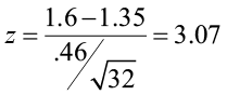
Step 3) Compute the test statistic.
- The test statistic is the number of standard deviations the sample mean is from the known mean. It is also a Z-score, just like the critical value.
-

- For this problem, the test statistic is
Step 4) State a conclusion.
- Compare the test statistic to the critical value. If the test statistic falls into the rejection zones, reject the null hypothesis. In other words, if the test statistic is greater than +1.96 or less than -1.96, reject the null hypothesis.
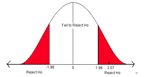
Figure 6. The critical values for a two-sided test when α = 0.05.
In this problem, the test statistic falls in the red rejection zone. The test statistic of 3.07 is greater than the critical value of 1.96.We will reject the null hypothesis. We have enough evidence to support the claim that the mean diameter growth is different from (not equal to) 1.35 in./year.
Example 7
A Right-sided Test
A researcher believes that there has been an increase in the average farm size in his state since the last study five years ago. The previous study reported a mean size of 450 acres with a population standard deviation (σ) of 167 acres. He samples 45 farms and gets a sample mean of 485.8 acres. Is there enough information to support his claim?
Step 1) State the null and alternative hypotheses.
- Ho: μ = 450 acres
- H1: μ >450 acres
Step 2) State the level of significance and the critical value.
- We will choose a level of significance of 5% (α = 0.05).
- For a one-sided question, we need a one-sided positive critical value Zα.
- The level of significance is all in the right side (the rejection zone is just on the right side).
- We need to find the Z-score associated with the 5% area in the right tail.
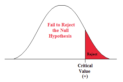
Figure 7. Rejection zone for a right-sided hypothesis test.
- Go into the body of values in the standard normal table and find the Z-score that separates the lower 95% from the upper 5%.
- The critical value is 1.645. This value sets up the rejection zone.
Step 3) Compute the test statistic.
- The test statistic is the number of standard deviations the sample mean is from the known mean. It is also a Z-score, just like the critical value.
-
- For this problem, the test statistic is
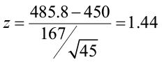
Step 4) State a conclusion.
- Compare the test statistic to the critical value.
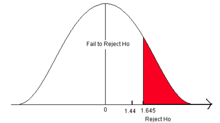
Figure 8. The critical value for a right-sided test when α = 0.05.
- The test statistic does not fall in the rejection zone. It is less than the critical value.
We fail to reject the null hypothesis. We do not have enough evidence to support the claim that the mean farm size has increased from 450 acres.
Example 8
A Left-sided Test
A researcher believes that there has been a reduction in the mean number of hours that college students spend preparing for final exams. A national study stated that students at a 4-year college spend an average of 23 hours preparing for 5 final exams each semester with a population standard deviation of 7.3 hours. The researcher sampled 227 students and found a sample mean study time of 19.6 hours. Does this indicate that the average study time for final exams has decreased? Use a 1% level of significance to test this claim.
Step 1) State the null and alternative hypotheses.
- Ho: μ = 23 hours
- H1: μ < 23 hours
Step 2) State the level of significance and the critical value.
- This is a left-sided test so alpha (0.01) is all in the left tail.
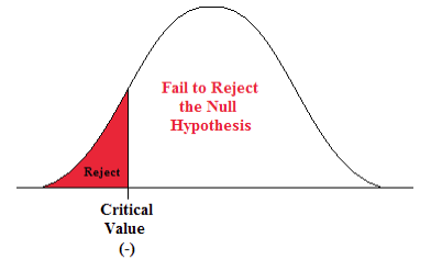
Figure 9. The rejection zone for a left-sided hypothesis test.
- Go into the body of values in the standard normal table and find the Z-score that defines the lower 1% of the area.
- The critical value is -2.33. This value sets up the rejection zone.
Step 3) Compute the test statistic.
- The test statistic is the number of standard deviations the sample mean is from the known mean. It is also a Z-score, just like the critical value.
-

- For this problem, the test statistic is
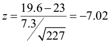
Step 4) State a conclusion.
- Compare the test statistic to the critical value.
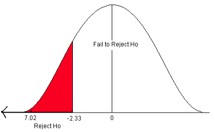
Figure 10. The critical value for a left-sided test when α = 0.01.
- The test statistic falls in the rejection zone. The test statistic of -7.02 is less than the critical value of -2.33.
We reject the null hypothesis. We have sufficient evidence to support the claim that the mean final exam study time has decreased below 23 hours.
Testing a Hypothesis using P-values
The p-value is the probability of observing our sample mean given that the null hypothesis is true. It is the area under the curve to the left or right of the test statistic. If the probability of observing such a sample mean is very small (less than the level of significance), we would reject the null hypothesis. Computations for the p-value depend on whether it is a one- or two-sided test.
Steps for a hypothesis test using p-values:
- State the null and alternative hypotheses.
- State the level of significance.
- Compute the test statistic and find the area associated with it (this is the p-value).
- Compare the p-value to alpha (α) and state a conclusion.
Instead of comparing Z-score test statistic to Z-score critical value, as in the classical method, we compare area of the test statistic to area of the level of significance.
The Decision Rule: If the p-value is less than alpha, we reject the null hypothesis
Computing P-values
If it is a two-sided test (the alternative claim is ≠), the p-value is equal to two times the probability of the absolute value of the test statistic. If the test is a left-sided test (the alternative claim is “<”), then the p-value is equal to the area to the left of the test statistic. If the test is a right-sided test (the alternative claim is “>”), then the p-value is equal to the area to the right of the test statistic.
Let’s look at Example 6 again.
A forester studying diameter growth of red pine believes that the mean diameter growth will be different from the known mean growth of 1.35 in./year if a fertilization treatment is applied to the stand. He conducts his experiment, collects data from a sample of 32 plots, and gets a sample mean diameter growth of 1.6 in./year. The population standard deviation for this stand is known to be 0.46 in./year. Does he have enough evidence to support his claim?
Step 1) State the null and alternative hypotheses.
- Ho: μ = 1.35 in./year
- H1: μ ≠ 1.35 in./year
Step 2) State the level of significance.
- We will choose a level of significance of 5% (α = 0.05).
Step 3) Compute the test statistic.
- For this problem, the test statistic is:

The p-value is two times the area of the absolute value of the test statistic (because the alternative claim is “not equal”).
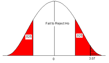
Figure 11. The p-value compared to the level of significance.
- Look up the area for the Z-score 3.07 in the standard normal table. The area (probability) is equal to 1 – 0.9989 = 0.0011.
- Multiply this by 2 to get the p-value = 2 * 0.0011 = 0.0022.
Step 4) Compare the p-value to alpha and state a conclusion.
- Use the Decision Rule (if the p-value is less than α, reject H0).
- In this problem, the p-value (0.0022) is less than alpha (0.05).
- We reject the H0. We have enough evidence to support the claim that the mean diameter growth is different from 1.35 inches/year.
Let’s look at Example 7 again.
A researcher believes that there has been an increase in the average farm size in his state since the last study five years ago. The previous study reported a mean size of 450 acres with a population standard deviation (σ) of 167 acres. He samples 45 farms and gets a sample mean of 485.8 acres. Is there enough information to support his claim?
Step 1) State the null and alternative hypotheses.
- Ho: μ = 450 acres
- H1: μ >450 acres
Step 2) State the level of significance.
- We will choose a level of significance of 5% (α = 0.05).
Step 3) Compute the test statistic.
- For this problem, the test statistic is
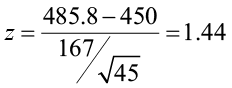
The p-value is the area to the right of the Z-score 1.44 (the hatched area).
- This is equal to 1 – 0.9251 = 0.0749.
- The p-value is 0.0749.
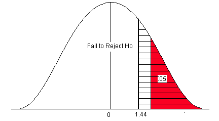
Figure 12. The p-value compared to the level of significance for a right-sided test.
Step 4) Compare the p-value to alpha and state a conclusion.
- Use the Decision Rule.
- In this problem, the p-value (0.0749) is greater than alpha (0.05), so we Fail to Reject the H0.
- The area of the test statistic is greater than the area of alpha (α).
We fail to reject the null hypothesis. We do not have enough evidence to support the claim that the mean farm size has increased.
Let’s look at Example 8 again.
A researcher believes that there has been a reduction in the mean number of hours that college students spend preparing for final exams. A national study stated that students at a 4-year college spend an average of 23 hours preparing for 5 final exams each semester with a population standard deviation of 7.3 hours. The researcher sampled 227 students and found a sample mean study time of 19.6 hours. Does this indicate that the average study time for final exams has decreased? Use a 1% level of significance to test this claim.
Step 1) State the null and alternative hypotheses.
- H0: μ = 23 hours
- H1: μ < 23 hours
Step 2) State the level of significance.
- This is a left-sided test so alpha (0.01) is all in the left tail.
Step 3) Compute the test statistic.
- For this problem, the test statistic is

The p-value is the area to the left of the test statistic (the little black area to the left of -7.02). The Z-score of -7.02 is not on the standard normal table. The smallest probability on the table is 0.0002. We know that the area for the Z-score -7.02 is smaller than this area (probability). Therefore, the p-value is <0.0002.
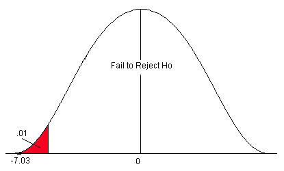
Figure 13. The p-value compared to the level of significance for a left-sided test.
Step 4) Compare the p-value to alpha and state a conclusion.
- Use the Decision Rule.
- In this problem, the p-value (p<0.0002) is less than alpha (0.01), so we Reject the H0.
- The area of the test statistic is much less than the area of alpha (α).
We reject the null hypothesis. We have enough evidence to support the claim that the mean final exam study time has decreased below 23 hours.
Both the classical method and p-value method for testing a hypothesis will arrive at the same conclusion. In the classical method, the critical Z-score is the number on the z-axis that defines the level of significance (α). The test statistic converts the sample mean to units of standard deviation (a Z-score). If the test statistic falls in the rejection zone defined by the critical value, we will reject the null hypothesis. In this approach, two Z-scores, which are numbers on the z-axis, are compared. In the p-value approach, the p-value is the area associated with the test statistic. In this method, we compare α (which is also area under the curve) to the p-value. If the p-value is less than α, we reject the null hypothesis. The p-value is the probability of observing such a sample mean when the null hypothesis is true. If the probability is too small (less than the level of significance), then we believe we have enough statistical evidence to reject the null hypothesis and support the alternative claim.
Software Solutions
Minitab
(referring to Ex. 8)
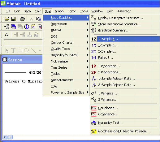

One-Sample Z
| Test of mu = 23 vs. < 23 |
| The assumed standard deviation = 7.3 |
| 99% Upper | |||||
| N | Mean | SE Mean | Bound | Z | P |
| 227 | 19.600 | 0.485 | 20.727 | -7.02 | 0.000 |
Excel
Excel does not offer 1-sample hypothesis testing.
Section 3
Hypothesis Test about the Population Mean (μ) when the Population Standard Deviation (σ) is Unknown
Frequently, the population standard deviation (σ) is not known. We can estimate the population standard deviation (σ) with the sample standard deviation (s). However, the test statistic will no longer follow the standard normal distribution. We must rely on the student’s t-distribution with n-1 degrees of freedom. Because we use the sample standard deviation (s), the test statistic will change from a Z-score to a t-score.
 →
→ 
Steps for a hypothesis test are the same that we covered in Section 2.
- State the null and alternative hypotheses.
- State the level of significance and the critical value.
- Compute the test statistic.
- State a conclusion.
Just as with the hypothesis test from the previous section, the data for this test must be from a random sample and requires either that the population from which the sample was drawn be normal or that the sample size is sufficiently large (n≥30). A t-test is robust, so small departures from normality will not adversely affect the results of the test. That being said, if the sample size is smaller than 30, it is always good to verify the assumption of normality through a normal probability plot.
We will still have the same three pairs of null and alternative hypotheses and we can still use either the classical approach or the p-value approach.
Selecting the correct critical value from the student’s t-distribution table depends on three factors: the type of test (one-sided or two-sided alternative hypothesis), the sample size, and the level of significance.
For a two-sided test (“not equal” alternative hypothesis), the critical value (tα/2), is determined by alpha (α), the level of significance, divided by two, to deal with the possibility that the result could be less than OR greater than the known value.
- If your level of significance was 0.05, you would use the 0.025 column to find the correct critical value (0.05/2 = 0.025).
- If your level of significance was 0.01, you would use the 0.005 column to find the correct critical value (0.01/2 = 0.005).
For a one-sided test (“a less than” or “greater than” alternative hypothesis), the critical value (tα) , is determined by alpha (α), the level of significance, being all in the one side.
- If your level of significance was 0.05, you would use the 0.05 column to find the correct critical value for either a left or right-side question. If you are asking a “less than” (left-sided question, your critical value will be negative. If you are asking a “greater than” (right-sided question), your critical value will be positive.
Example 9
Find the critical value you would use to test the claim that μ ≠ 112 with a sample size of 18 and a 5% level of significance.
In this case, the critical value (tα/2) would be 2.110. This is a two-sided question (≠) so you would divide alpha by 2 (0.05/2 = 0.025) and go down the 0.025 column to 17 degrees of freedom.
Example 10
What would the critical value be if you wanted to test that μ < 112 for the same data?
In this case, the critical value would be 1.740. This is a one-sided question (<) so alpha would be divided by 1 (0.05/1 = 0.05). You would go down the 0.05 column with 17 degrees of freedom to get the correct critical value.
Example 11
A Two-sided Test
In 2005, the mean pH level of rain in a county in northern New York was 5.41. A biologist believes that the rain acidity has changed. He takes a random sample of 11 rain dates in 2010 and obtains the following data. Use a 1% level of significance to test his claim.
4.70, 5.63, 5.02, 5.78, 4.99, 5.91, 5.76, 5.54, 5.25, 5.18, 5.01
The sample size is small and we don’t know anything about the distribution of the population, so we examine a normal probability plot. The distribution looks normal so we will continue with our test.
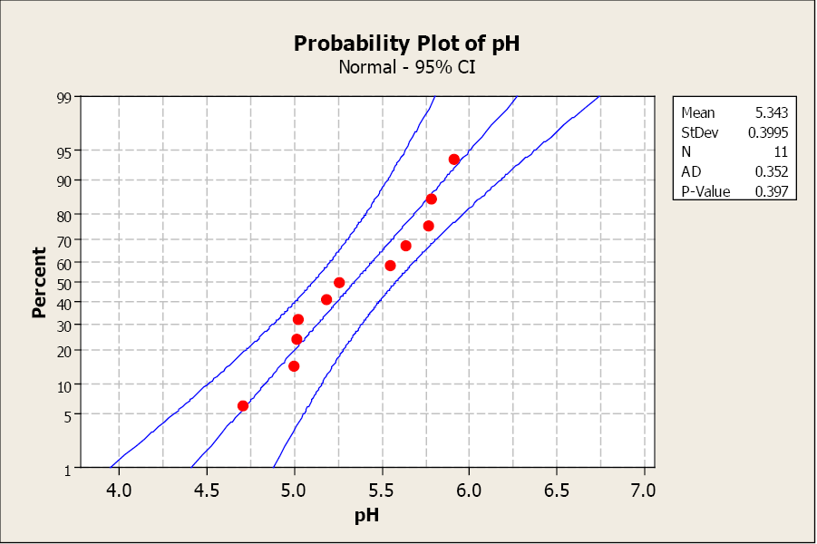
Figure 14. A normal probability plot for Example 9.
The sample mean is 5.343 with a sample standard deviation of 0.397.
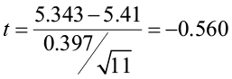
Step 1) State the null and alternative hypotheses.
- Ho: μ = 5.41
- H1: μ ≠ 5.41
Step 2) State the level of significance and the critical value.
- This is a two-sided question so alpha is divided by two.
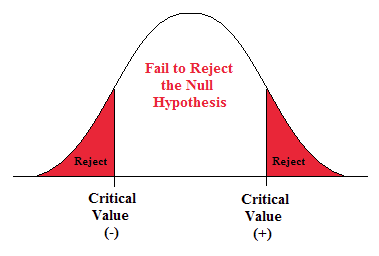
Figure 15. The rejection zones for a two-sided test.
- t α/2 is found by going down the 0.005 column with 14 degrees of freedom.
- t α/2 = ±3.169.
Step 3) Compute the test statistic.
- The test statistic is a t-score.

- For this problem, the test statistic is
Step 4) State a conclusion.
- Compare the test statistic to the critical value.
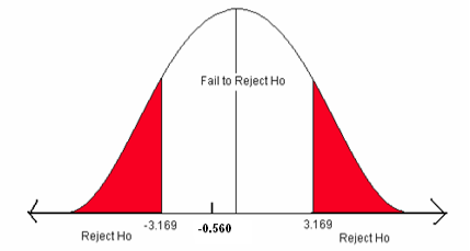
Figure 16. The critical values for a two-sided test when α = 0.01.
- The test statistic does not fall in the rejection zone.
We will fail to reject the null hypothesis. We do not have enough evidence to support the claim that the mean rain pH has changed.
Example 12
A One-sided Test
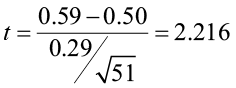
Cadmium, a heavy metal, is toxic to animals. Mushrooms, however, are able to absorb and accumulate cadmium at high concentrations. The government has set safety limits for cadmium in dry vegetables at 0.5 ppm. Biologists believe that the mean level of cadmium in mushrooms growing near strip mines is greater than the recommended limit of 0.5 ppm, negatively impacting the animals that live in this ecosystem. A random sample of 51 mushrooms gave a sample mean of 0.59 ppm with a sample standard deviation of 0.29 ppm. Use a 5% level of significance to test the claim that the mean cadmium level is greater than the acceptable limit of 0.5 ppm.
The sample size is greater than 30 so we are assured of a normal distribution of the means.
Step 1) State the null and alternative hypotheses.
- Ho: μ = 0.5 ppm
- H1: μ > 0.5 ppm
Step 2) State the level of significance and the critical value.
- This is a right-sided question so alpha is all in the right tail.
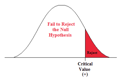
Figure 17. Rejection zone for a right-sided test.
- t α is found by going down the 0.05 column with 50 degrees of freedom.
- t α = 1.676
Step 3) Compute the test statistic.
- The test statistic is a t-score.

- For this problem, the test statistic is
Step 4) State a Conclusion.
- Compare the test statistic to the critical value.
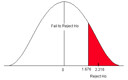
Figure 18. Critical value for a right-sided test when α = 0.05.
The test statistic falls in the rejection zone. We will reject the null hypothesis. We have enough evidence to support the claim that the mean cadmium level is greater than the acceptable safe limit.
BUT, what happens if the significance level changes to 1%?
The critical value is now found by going down the 0.01 column with 50 degrees of freedom. The critical value is 2.403. The test statistic is now LESS THAN the critical value. The test statistic does not fall in the rejection zone. The conclusion will change. We do NOT have enough evidence to support the claim that the mean cadmium level is greater than the acceptable safe limit of 0.5 ppm.
The level of significance is the probability that you, as the researcher, set to decide if there is enough statistical evidence to support the alternative claim. It should be set before the experiment begins.
P-value Approach
We can also use the p-value approach for a hypothesis test about the mean when the population standard deviation (σ) is unknown. However, when using a student’s t-table, we can only estimate the range of the p-value, not a specific value as when using the standard normal table. The student’s t-table has area (probability) across the top row in the table, with t-scores in the body of the table.
- To find the p-value (the area associated with the test statistic), you would go to the row with the number of degrees of freedom.
- Go across that row until you find the two values that your test statistic is between, then go up those columns to find the estimated range for the p-value.
Example 13
Estimating P-value from a Student’s T-table
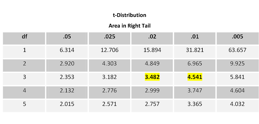 Table 3. Portion of the student’s t-table.
If your test statistic is 3.789 with 3 degrees of freedom, you would go across the 3 df row. The value 3.789 falls between the values 3.482 and 4.541 in that row. Therefore, the p-value is between 0.02 and 0.01. The p-value will be greater than 0.01 but less than 0.02 (0.01<p<0.02).
Conclusion
If your level of significance is 5%, you would reject the null hypothesis as the p-value (0.01-0.02) is less than alpha (α) of 0.05.
If your level of significance is 1%, you would fail to reject the null hypothesis as the p-value (0.01-0.02) is greater than alpha (α) of 0.01.
Software packages typically output p-values. It is easy to use the Decision Rule to answer your research question by the p-value method.
Software Solutions
Minitab
(referring to Ex. 12)

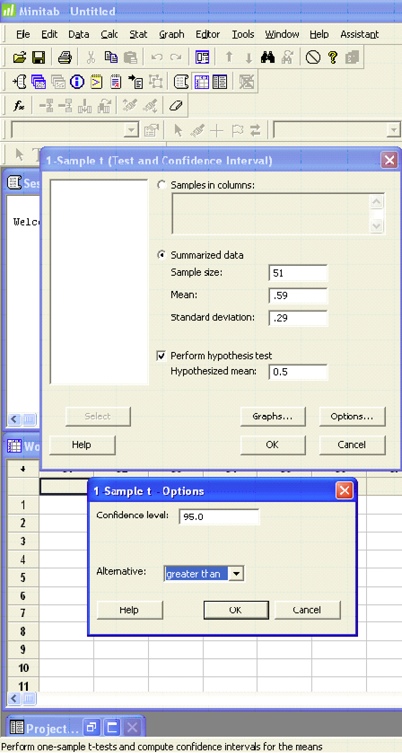
One-Sample T
Test of mu = 0.5 vs. > 0.5
|
95% Lower |
||||||
|
N |
Mean |
StDev |
SE Mean |
Bound |
T |
P |
|
51 |
0.5900 |
0.2900 |
0.0406 |
0.5219 |
2.22 |
0.016 |
Additional example: www.youtube.com/watch?v=WwdSjO4VUsg.
Excel
Excel does not offer 1-sample hypothesis testing.
Section 4
Hypothesis Test for a Population Proportion (p)
Frequently, the parameter we are testing is the population proportion.
- We are studying the proportion of trees with cavities for wildlife habitat.
- We need to know if the proportion of people who support green building materials has changed.
- Has the proportion of wolves that died last year in Yellowstone increased from the year before?
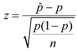
Recall that the best point estimate of p, the population proportion, is given by

where x is the number of individuals in the sample with the characteristic studied and n is the sample size. The sampling distribution of p̂ is approximately normal with a mean ![]() and a standard deviation
and a standard deviation
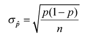
when np(1 – p)≥10. We can use both the classical approach and the p-value approach for testing.
The steps for a hypothesis test are the same that we covered in Section 2.
- State the null and alternative hypotheses.
- State the level of significance and the critical value.
- Compute the test statistic.
- State a conclusion.
The test statistic follows the standard normal distribution. Notice that the standard error (the denominator) uses p instead of p̂, which was used when constructing a confidence interval about the population proportion. In a hypothesis test, the null hypothesis is assumed to be true, so the known proportion is used.

- The critical value comes from the standard normal table, just as in Section 2. We will still use the same three pairs of null and alternative hypotheses as we used in the previous sections, but the parameter is now p instead of μ:
- For a two-sided test, alpha will be divided by 2 giving a ± Zα/2 critical value.
- For a left-sided test, alpha will be all in the left tail giving a – Zα critical value.
- For a right-sided test, alpha will be all in the right tail giving a Zα critical value.
Example 14
A botanist has produced a new variety of hybrid soy plant that is better able to withstand drought than other varieties. The botanist knows the seed germination for the parent plants is 75%, but does not know the seed germination for the new hybrid. He tests the claim that it is different from the parent plants. To test this claim, 450 seeds from the hybrid plant are tested and 321 have germinated. Use a 5% level of significance to test this claim that the germination rate is different from 75%.
Step 1) State the null and alternative hypotheses.
- Ho: p = 0.75
- H1: p ≠ 0.75
Step 2) State the level of significance and the critical value.
This is a two-sided question so alpha is divided by 2.
- Alpha is 0.05 so the critical values are ± Zα/2 = ± Z.025.
- Look on the negative side of the standard normal table, in the body of values for 0.025.
- The critical values are ± 1.96.
Step 3) Compute the test statistic.
- The test statistic is the number of standard deviations the sample mean is from the known mean. It is also a Z-score, just like the critical value.
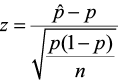
- For this problem, the test statistic is
Step 4) State a conclusion.
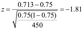
- Compare the test statistic to the critical value.
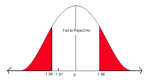
Figure 19. Critical values for a two-sided test when α = 0.05.
The test statistic does not fall in the rejection zone. We fail to reject the null hypothesis. We do not have enough evidence to support the claim that the germination rate of the hybrid plant is different from the parent plants.
Let’s answer this question using the p-value approach. Remember, for a two-sided alternative hypothesis (“not equal”), the p-value is two times the area of the test statistic. The test statistic is -1.81 and we want to find the area to the left of -1.81 from the standard normal table.
- On the negative page, find the Z-score -1.81. Find the area associated with this Z-score.
- The area = 0.0351.
- This is a two-sided test so multiply the area times 2 to get the p-value = 0.0351 x 2 = 0.0702.
Now compare the p-value to alpha. The Decision Rule states that if the p-value is less than alpha, reject the H0. In this case, the p-value (0.0702) is greater than alpha (0.05) so we will fail to reject H0. We do not have enough evidence to support the claim that the germination rate of the hybrid plant is different from the parent plants.
Example 15
You are a biologist studying the wildlife habitat in the Monongahela National Forest. Cavities in older trees provide excellent habitat for a variety of birds and small mammals. A study five years ago stated that 32% of the trees in this forest had suitable cavities for this type of wildlife. You believe that the proportion of cavity trees has increased. You sample 196 trees and find that 79 trees have cavities. Does this evidence support your claim that there has been an increase in the proportion of cavity trees?
Use a 10% level of significance to test this claim.
Step 1) State the null and alternative hypotheses.
- Ho: p = 0.32
- H1: p > 0.32
Step 2) State the level of significance and the critical value.
This is a one-sided question so alpha is divided by 1.
- Alpha is 0.10 so the critical value is Zα = Z .10
- Look on the positive side of the standard normal table, in the body of values for 0.90.
- The critical value is 1.28.
Figure 20. Critical value for a right-sided test where α = 0.10.
Step 3) Compute the test statistic.
- The test statistic is the number of standard deviations the sample proportion is from the known proportion. It is also a Z-score, just like the critical value.

- For this problem, the test statistic is:
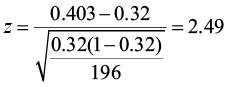
Step 4) State a conclusion.
- Compare the test statistic to the critical value.
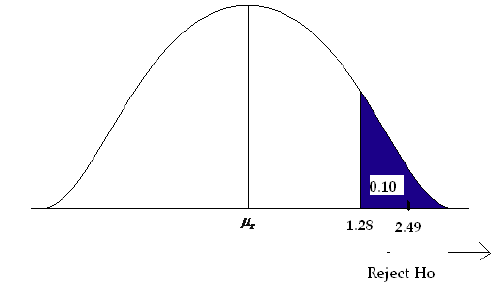
Figure 21. Comparison of the test statistic and the critical value.
The test statistic is larger than the critical value (it falls in the rejection zone). We will reject the null hypothesis. We have enough evidence to support the claim that there has been an increase in the proportion of cavity trees.
Now use the p-value approach to answer the question. This is a right-sided question (“greater than”), so the p-value is equal to the area to the right of the test statistic. Go to the positive side of the standard normal table and find the area associated with the Z-score of 2.49. The area is 0.9936. Remember that this table is cumulative from the left. To find the area to the right of 2.49, we subtract from one.
p-value = (1 – 0.9936) = 0.0064
The p-value is less than the level of significance (0.10), so we reject the null hypothesis. We have enough evidence to support the claim that the proportion of cavity trees has increased.
Software Solutions
Minitab
(referring to Ex. 15)


Test and CI for One Proportion
Test of p = 0.32 vs. p > 0.32
|
90% Lower |
||||||
| Sample | X | N | Sample p | Bound | Z-Value | p-Value |
| 1 | 79 | 196 | 0.403061 | 0.358160 | 2.49 | 0.006 |
| Using the normal approximation. | ||||||
Excel
Excel does not offer 1-sample hypothesis testing.
Section 5
Hypothesis Test about a Variance
When people think of statistical inference, they usually think of inferences involving population means or proportions. However, the particular population parameter needed to answer an experimenter’s practical questions varies from one situation to another, and sometimes a population’s variability is more important than its mean. Thus, product quality is often defined in terms of low variability.
Sample variance S2 can be used for inferences concerning a population variance σ2. For a random sample of n measurements drawn from a normal population with mean μ and variance σ2, the value S2 provides a point estimate for σ2. In addition, the quantity (n – 1)S2 / σ2 follows a Chi-square (χ2) distribution, with df = n – 1.
The properties of Chi-square (χ2) distribution are:
- Unlike Z and t distributions, the values in a chi-square distribution are all positive.
- The chi-square distribution is asymmetric, unlike the Z and t distributions.
- There are many chi-square distributions. We obtain a particular one by specifying the degrees of freedom (df = n – 1) associated with the sample variances S2.
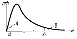
Figure 22. The chi-square distribution.
One-sample χ2 test for testing the hypotheses:
Null hypothesis: H0: σ2 =  (constant)
Alternative hypothesis:
- Ha: σ2 >
 (one-tailed), reject H0 if the observed χ2 >
  (upper-tail value at α).
 - Ha: σ2 <
 (one-tailed), reject H0 if the observed χ2 <
  (lower-tail value at α).
 - Ha: σ2 ≠
 (two-tailed), reject H0 if the observed χ2 >
  or χ2 <
  at α/2.
where the χ2 critical value in the rejection region is based on degrees of freedom df = n – 1 and a specified significance level of α.
Test statistic: 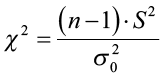 .
.
As with previous sections, if the test statistic falls in the rejection zone set by the critical value, you will reject the null hypothesis.
Example 16
A forester wants to control a dense understory of striped maple that is interfering with desirable hardwood regeneration using a mist blower to apply an herbicide treatment. She wants to make sure that treatment has a consistent application rate, in other words, low variability not exceeding 0.25 gal./acre (0.06 gal.2). She collects sample data (n = 11) on this type of mist blower and gets a sample variance of 0.064 gal.2 Using a 5% level of significance, test the claim that the variance is significantly greater than 0.06 gal.2
H0: σ2 = 0.06
H1: σ2 >0.06
The critical value is 18.307. Any test statistic greater than this value will cause you to reject the null hypothesis.
The test statistic is
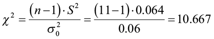
We fail to reject the null hypothesis. The forester does NOT have enough evidence to support the claim that the variance is greater than 0.06 gal.2 You can also estimate the p-value using the same method as for the student t-table. Go across the row for degrees of freedom until you find the two values that your test statistic falls between. In this case going across the row 10, the two table values are 4.865 and 15.987. Now go up those two columns to the top row to estimate the p-value (0.1-0.9). The p-value is greater than 0.1 and less than 0.9. Both are greater than the level of significance (0.05) causing us to fail to reject the null hypothesis.
Software Solutions
Minitab
(referring to Ex. 16)


Test and CI for One Variance
|
Method |
||
| Null hypothesis | Sigma-squared | = 0.06 |
| Alternative hypothesis | Sigma-squared | > 0.06 |
The chi-square method is only for the normal distribution.
Tests
|
Test |
|||
| Method | Statistic | DF | P-Value |
| Chi-Square | 10.67 | 10 | 0.384 |
Excel
Excel does not offer 1-sample χ2 testing.
Section 6
Putting it all Together Using the Classical Method
To Test a Claim about μ when σ is Known
- Write the null and alternative hypotheses.
- State the level of significance and get the critical value from the standard normal table.
- Compute the test statistic.

- Compare the test statistic to the critical value (Z-score) and write the conclusion.
To Test a Claim about μ When σ is Unknown
- Write the null and alternative hypotheses.
- State the level of significance and get the critical value from the student’s t-table with n-1 degrees of freedom.
- Compute the test statistic.

- Compare the test statistic to the critical value (t-score) and write the conclusion.
To Test a Claim about p
- Write the null and alternative hypotheses.
- State the level of significance and get the critical value from the standard normal distribution.
- Compute the test statistic.
- Compare the test statistic to the critical value (Z-score) and write the conclusion.

Table 4. A summary table for critical Z-scores.
To Test a Claim about Variance
- Write the null and alternative hypotheses.
- State the level of significance and get the critical value from the chi-square table using n-1 degrees of freedom.
- Compute the test statistic.

- Compare the test statistic to the critical value and write the conclusion.
Candela Citations
- Natural Resources Biometrics. Authored by: Diane Kiernan. Located at: https://textbooks.opensuny.org/natural-resources-biometrics/. Project: Open SUNY Textbooks. License: CC BY-NC-SA: Attribution-NonCommercial-ShareAlike