Sampling Distribution of the Sample Mean
Inferential testing uses the sample mean (x̄) to estimate the population mean (μ). Typically, we use the data from a single sample, but there are many possible samples of the same size that could be drawn from that population. As we saw in the previous chapter, the sample mean (x̄) is a random variable with its own distribution.
- The distribution of the sample mean will have a mean equal to µ.
- It will have a standard deviation (standard error) equal to

Because our inferences about the population mean rely on the sample mean, we focus on the distribution of the sample mean. Is it normal? What if our population is not normally distributed or we don’t know anything about the distribution of our population?
The Central Limit Theorem states that the sampling distribution of the sample means will approach a normal distribution as the sample size increases.
- So if we do not have a normal distribution, or know nothing about our distribution, the CLT tells us that the distribution of the sample means (x̄) will become normal distributed as n (sample size) increases.
- How large does n have to be?
- A general rule of thumb tells us that n ≥ 30.
The Central Limit Theorem tells us that regardless of the shape of our population, the sampling distribution of the sample mean will be normal as the sample size increases.
Sampling Distribution of the Sample Proportion
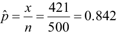
The population proportion (p) is a parameter that is as commonly estimated as the mean. It is just as important to understand the distribution of the sample proportion, as the mean. With proportions, the element either has the characteristic you are interested in or the element does not have the characteristic. The sample proportion (p̂) is calculated by

where x is the number of elements in your population with the characteristic and n is the sample size.
Example 1
You are studying the number of cavity trees in the Monongahela National Forest for wildlife habitat. You have a sample size of n = 950 trees and, of those trees, x = 238 trees with cavities. The sample proportion is:
The distribution of the sample proportion has a mean of ![]()
and has a standard deviation of 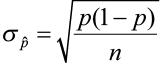 .
.
The sample proportion is normally distributed if n is very large and ![]() isn’t close to 0 or 1. We can also use the following relationship to assess normality when the parameter being estimated is p, the population proportion:
isn’t close to 0 or 1. We can also use the following relationship to assess normality when the parameter being estimated is p, the population proportion:
Confidence Intervals
In the preceding chapter we learned that populations are characterized by descriptive measures called parameters. Inferences about parameters are based on sample statistics. We now want to estimate population parameters and assess the reliability of our estimates based on our knowledge of the sampling distributions of these statistics.
Point Estimates
We start with a point estimate. This is a single value computed from the sample data that is used to estimate the population parameter of interest.
- The sample mean (x̄) is a point estimate of the population mean (μ).
- The sample proportion (p̂) is the point estimate of the population proportion (p).
We use point estimates to construct confidence intervals for unknown parameters.
- A confidence interval is an interval of values instead of a single point estimate.
- The level of confidence corresponds to the expected proportion of intervals that will contain the parameter if many confidence intervals are constructed of the same sample size from the same population.
- Our uncertainty is about whether our particular confidence interval is one of those that truly contains the true value of the parameter.
Example 2
We are 95% confident that our interval contains the population mean bear weight.
If we created 100 confidence intervals of the same size from the same population, we would expect 95 of them to contain the true parameter (the population mean weight). We also expect five of the intervals would not contain the parameter.
Figure 1. Confidence intervals from twenty-five different samples.
In this example, twenty-five samples from the same population gave these 95% confidence intervals. In the long term, 95% of all samples give an interval that contains µ, the true (but unknown) population mean.
Level of confidence is expressed as a percent.
- The compliment to the level of confidence is α (alpha), the level of significance.
- The level of confidence is described as (1- α) * 100%.
What does this really mean?
- We use a point estimate (e.g., sample mean) to estimate the population mean.
- We attach a level of confidence to this interval to describe how certain we are that this interval actually contains the unknown population parameter.
- We want to estimate the population parameter, such as the mean (μ) or proportion (p).
 < μ <
< μ <  or
or  < p <
< p < 
where E is the margin of error.
The confidence is based on area under a normal curve. So the assumption of normality must be met (see Chapter 1).
Confidence Intervals about the Mean (μ) when the Population Standard Deviation (σ) is Known
A confidence interval takes the form of: point estimate ± margin of error.
The point estimate
- The point estimate comes from the sample data.
- To estimate the population mean (μ), use the sample mean (x̄) as the point estimate.
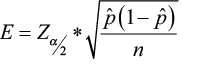
The margin of error
- Depends on the level of confidence, the sample size and the population standard deviation.
- It is computed as
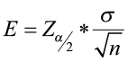 where
where  is the critical value from the standard normal table associated with α (the level of significance).
The critical value 
- This is a Z-score that bounds the level of confidence.
- Confidence intervals are ALWAYS two-sided and the Z-scores are the limits of the area associated with the level of confidence.
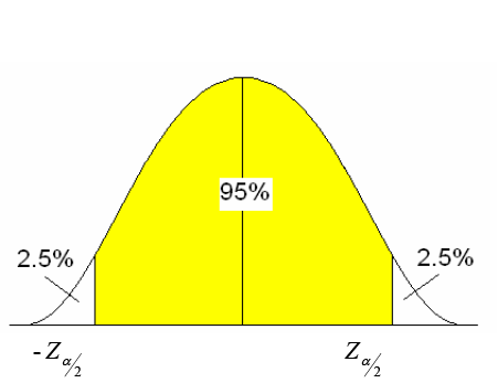
Figure 2. The middle 95% area under a standard normal curve.
- The level of significance (α) is divided into halves because we are looking at the middle 95% of the area under the curve.
- Go to your standard normal table and find the area of 0.025 in the body of values.
- What is the Z-score for that area?
- The Z-scores of ± 1.96 are the critical Z-scores for a 95% confidence interval.
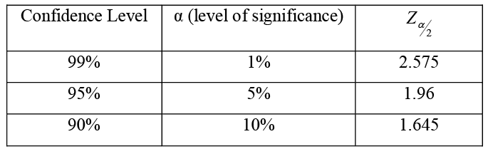
Table 1. Common critical values (Z-scores).
Construction of a confidence interval about μ when σ is known:
 (critical value)
 (margin of error)
 (point estimate ± margin of error)
Example 3
Construct a confidence interval about the population mean.
Researchers have been studying p-loading in Jones Lake for many years. It is known that mean water clarity (using a Secchi disk) is normally distributed with a population standard deviation of σ = 15.4 in. A random sample of 22 measurements was taken at various points on the lake with a sample mean of x̄ = 57.8 in. The researchers want you to construct a 95% confidence interval for μ, the mean water clarity.
1) ![]() = 1.96
= 1.96
2)  =
= 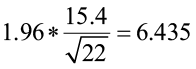
3) ![]() = 57.8 ± 6.435
= 57.8 ± 6.435
95% confidence interval for the mean water clarity is (51.36, 64.24).
We can be 95% confident that this interval contains the population mean water clarity for Jones Lake.
Now construct a 99% confidence interval for μ, the mean water clarity, and interpret.
1) ![]() = 2.575
= 2.575
2)  =
= 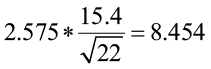
3) ![]() = 57.8± 8.454
= 57.8± 8.454
99% confidence interval for the mean water clarity is (49.35, 66.25).
We can be 99% confident that this interval contains the population mean water clarity for Jones Lake.
As the level of confidence increased from 95% to 99%, the width of the interval increased. As the probability (area under the normal curve) increased, the critical value increased resulting in a wider interval.
Software Solutions
Minitab
You can use Minitab to construct this 95% confidence interval (Excel does not construct confidence intervals about the mean when the population standard deviation is known). Select Basic Statistics>1-sample Z. Enter the known population standard deviation and select the required level of confidence.
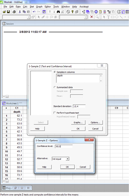
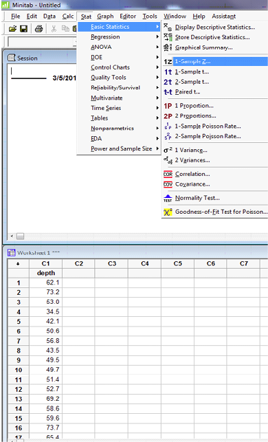
Figure 3. Minitab screen shots for constructing a confidence interval.
One-Sample Z: depth
|
The assumed standard deviation = 15.4 |
|||||
|
Variable |
N |
Mean |
StDev |
SE Mean |
95% CI |
|
depth |
22 |
57.80 |
11.60 |
3.28 |
(51.36, 64.24) |
Confidence Intervals about the Mean (μ) when the Population Standard Deviation (σ) is Unknown
Typically, in real life we often don’t know the population standard deviation (σ). We can use the sample standard deviation (s) in place of σ. However, because of this change, we can’t use the standard normal distribution to find the critical values necessary for constructing a confidence interval.
The Student’s t-distribution was created for situations when σ was unknown. Gosset worked as a quality control engineer for Guinness Brewery in Dublin. He found errors in his testing and he knew it was due to the use of s instead of σ. He created this distribution to deal with the problem of an unknown population standard deviation and small sample sizes. A portion of the t-table is shown below.
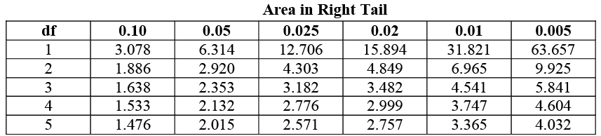
Table 2. Portion of the student’s t-table.
Example 4
Find the critical value ![]() for a 95% confidence interval with a sample size of n=13.
for a 95% confidence interval with a sample size of n=13.
- Degrees of freedom (down the left-hand column) is equal to n-1 = 12
- α = 0.05 and α/2 = 0.025
- Go down the 0.025 column to 12 df
 = 2.179
The critical values from the students’ t-distribution approach the critical values from the standard normal distribution as the sample size (n) increases.
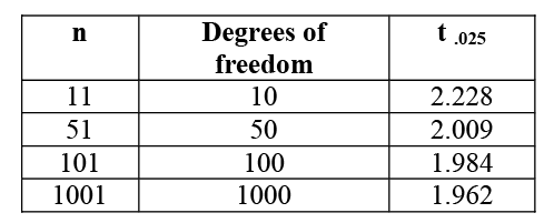
Table 3. Critical values from the student’s t-table.
Using the standard normal curve, the critical value for a 95% confidence interval is 1.96. You can see how different samples sizes will change the critical value and thus the confidence interval, especially when the sample size is small.
Construction of a Confidence Interval about μ when σ is Unknown
 critical value with n-1 df
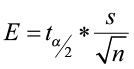

Example 5
Researchers studying the effects of acid rain in the Adirondack Mountains collected water samples from 22 lakes. They measured the pH (acidity) of the water and want to construct a 99% confidence interval about the mean lake pH for this region. The sample mean is 6.4438 with a sample standard deviation of 0.7120. They do not know anything about the distribution of the pH of this population, and the sample is small (n<30), so they look at a normal probability plot.
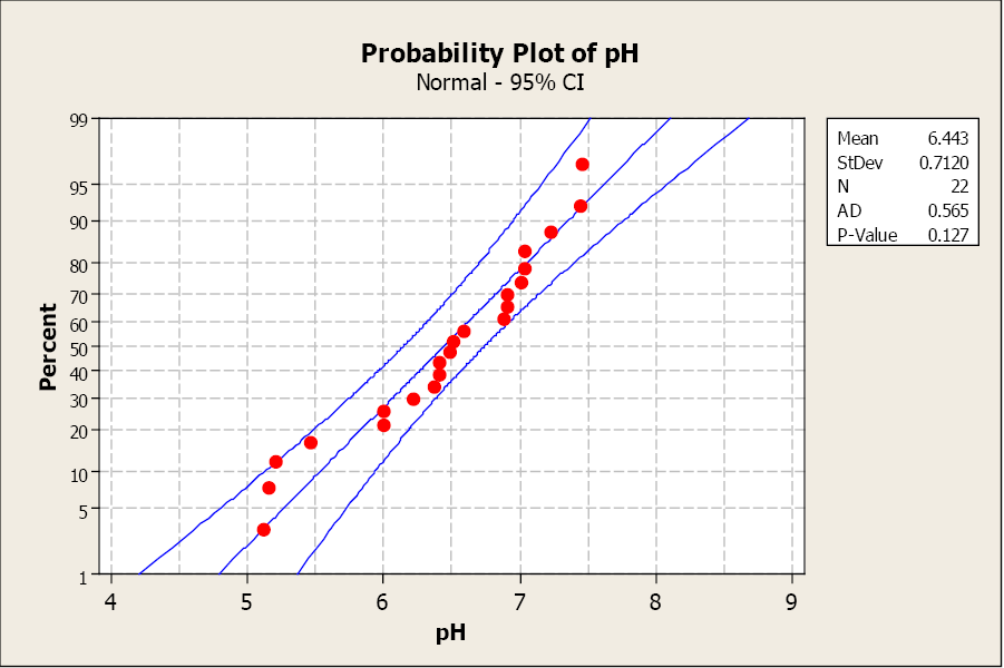
Figure 4. Normal probability plot.
The data is normally distributed. Now construct the 99% confidence interval about the mean pH.
1) ![]() = 2.831
= 2.831
2)  =
= 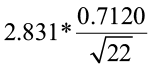 = 0.4297
3) ![]() = 6.443 ± 0.4297
= 6.443 ± 0.4297
The 99% confidence interval about the mean pH is (6.013, 6.863).
We are 99% confident that this interval contains the mean lake pH for this lake population.
Now construct a 90% confidence interval about the mean pH for these lakes.
1) ![]() = 1.721
= 1.721
2)  =
= 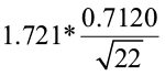 = 0.2612
3) ![]() = 6.443 ± 0.2612
= 6.443 ± 0.2612
The 90% confidence interval about the mean pH is (6.182, 6.704).
We are 90% confident that this interval contains the mean lake pH for this lake population.
Notice how the width of the interval decreased as the level of confidence decreased from 99 to 90%.
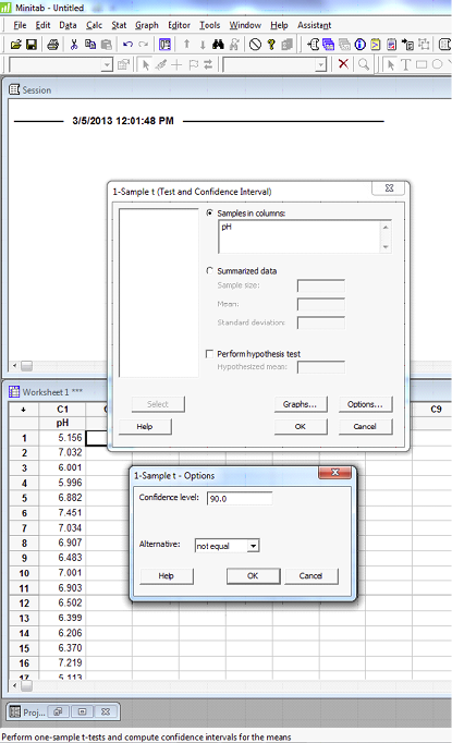
Construct a 90% confidence interval about the mean lake pH using Excel and Minitab.
Software Solutions
Minitab
For Minitab, enter the data in the spreadsheet and select Basic statistics and 1-sample t-test.
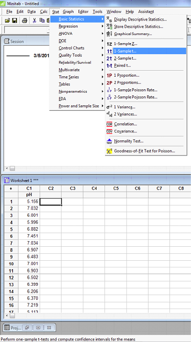
One-Sample T: pH
| Variable | N | Mean | StDev | SE Mean | 90% CI |
| pH |
22 |
6.443 |
0.712 |
0.152 |
(6.182, 6.704) |
Additional example:
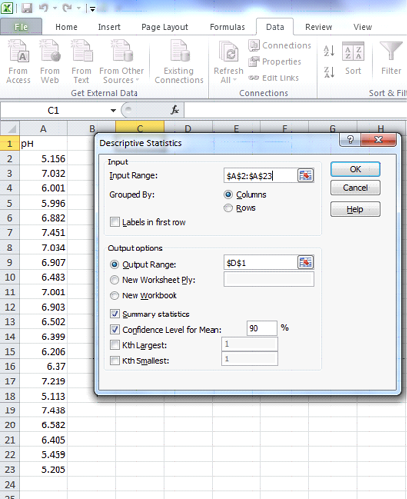
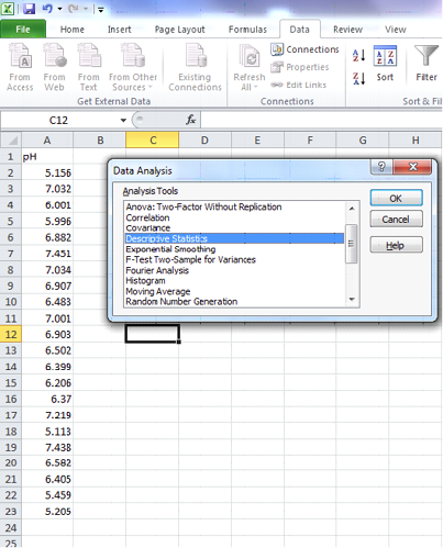
For Excel, enter the data in the spreadsheet and select descriptive statistics. Check Summary Statistics and select the level and confidence.Excel
|
Mean |
6.442909 |
|
Standard Error |
0.151801 |
|
Median |
6.4925 |
|
Mode |
#N/A |
|
Standard Deviation |
0.712008 |
|
Sample Variance |
0.506956 |
|
Kurtosis |
-0.5007 |
|
Skewness |
-0.60591 |
|
Range |
2.338 |
|
Minimum |
5.113 |
|
Maximum |
7.451 |
|
Sum |
141.744 |
|
Count |
22 |
|
Confidence Level(90.0%) |
0.26121 |
Excel gives you the sample mean in the first line (6.442909) and the margin of error in the last line (0.26121). You must complete the computation yourself to obtain the interval (6.442909±0.26121).
Confidence Intervals about the Population Proportion (p)
Frequently, we are interested in estimating the population proportion (p), instead of the population mean (µ). For example, you may need to estimate the proportion of trees infected with beech bark disease, or the proportion of people who support “green” products. The parameter p can be estimated in the same ways as we estimated µ, the population mean.
The Sample Proportion
- The sample proportion is the best point estimate for the true population proportion.
- Sample proportion
 where x is the number of elements in the sample with the characteristic you are interested in, and n is the sample size.
The Assumption of Normality when Estimating Proportions
- The assumption of a normally distributed population is still important, even though the parameter has changed.
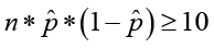
- Normality can be verified if:
-
Constructing a Confidence Interval about the Population Proportion
Constructing a confidence interval about the proportion follows the same three steps we have used in previous examples.
 (critical value from the standard normal table)
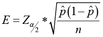 (margin of error)
 (point estimate ± margin of error)
Example 6
A botanist has produced a new variety of hybrid soybean that is better able to withstand drought. She wants to construct a 95% confidence interval about the germination rate (percent germination). She randomly selected 500 seeds and found that 421 have germinated.
First, compute the point estimate
Check normality: ![]()
You can assume a normal distribution.
Now construct the confidence interval:
1) ![]() = 1.96
= 1.96
2)  =
= 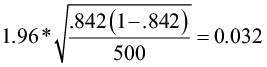
3) ![]()
The 95% confidence interval for the germination rate is (81.0%, 87.4%).
We can be 95% confident that this interval contains the true germination rate for this population.
Software Solutions
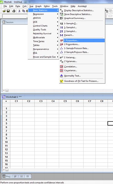
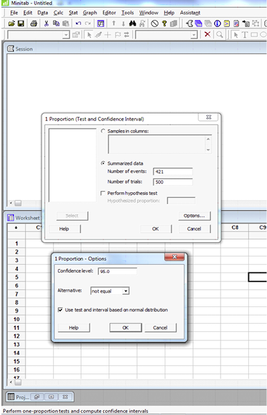
Minitab
You can use Minitab to compute the confidence interval. Select STAT>Basic stats>1-proportion. Select summarized data and enter the number of events (421) and the number of trials (500). Click Options and select the correct confidence level. Check “test and interval based on normal distribution” if the assumption of normality has been verified.
Test and CI for One Proportion
| Sample | X | N | Sample p | 95% CI |
| 1 | 421 | 500 | 0.842000 | (0.810030, 0.873970) |
Using the normal approximation.
Excel
Excel does not compute confidence intervals for estimating the population proportion.
Confidence Interval Summary
Which method do I use?
The first question to ask yourself is: Which parameter are you trying to estimate? If it is the mean (µ), then ask yourself: Is the population standard deviation (σ) known? If yes, then follow the next 3 steps:
Confidence Interval about the Population Mean (µ) when σ is Known
 critical value (from the standard normal table)

If no, follow these 3 steps:
Confidence Interval about the Population Mean (µ) when σ is Unknown
 critical value with n-1 df from the student t-distribution

If you want to construct a confidence interval about the population proportion, follow these 3 steps:
Confidence Interval about the Proportion
 critical value from the standard normal table

Remember that the assumption of normality must be verified.
Candela Citations
- Natural Resources Biometrics. Authored by: Diane Kiernan. Located at: https://textbooks.opensuny.org/natural-resources-biometrics/. Project: Open SUNY Textbooks. License: CC BY-NC-SA: Attribution-NonCommercial-ShareAlike