Learning Objectives
- Apply the formulas for derivatives and integrals of the hyperbolic functions.
- Apply the formulas for the derivatives of the inverse hyperbolic functions and their associated integrals.
- Describe the common applied conditions of a catenary curve.
We were introduced to hyperbolic functions in Introduction to Functions and Graphs, along with some of their basic properties. In this section, we look at differentiation and integration formulas for the hyperbolic functions and their inverses.
Derivatives and Integrals of the Hyperbolic Functions
Recall that the hyperbolic sine and hyperbolic cosine are defined as
The other hyperbolic functions are then defined in terms of [latex]\text{sinh}x[/latex] and [latex]\text{cosh}x.[/latex] The graphs of the hyperbolic functions are shown in the following figure.
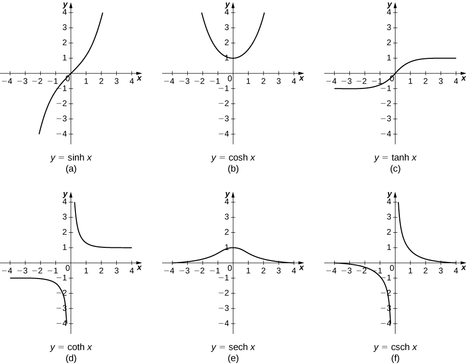
Figure 1. Graphs of the hyperbolic functions.
It is easy to develop differentiation formulas for the hyperbolic functions. For example, looking at [latex]\text{sinh}x[/latex] we have
Similarly, [latex](d\text{/}dx)\text{cosh}x=\text{sinh}x.[/latex] We summarize the differentiation formulas for the hyperbolic functions in the following table.
| [latex]f(x)[/latex] | [latex]\frac{d}{dx}f(x)[/latex] |
|---|---|
| [latex]\text{sinh}x[/latex] | [latex]\text{cosh}x[/latex] |
| [latex]\text{cosh}x[/latex] | [latex]\text{sinh}x[/latex] |
| [latex]\text{tanh}x[/latex] | [latex]{\text{sech}}^{2}x[/latex] |
| [latex]\text{coth}x[/latex] | [latex]\text{−}{\text{csch}}^{2}x[/latex] |
| [latex]\text{sech}x[/latex] | [latex]\text{−}\text{sech}x\text{tanh}x[/latex] |
| [latex]\text{csch}x[/latex] | [latex]\text{−}\text{csch}x\text{coth}x[/latex] |
Let’s take a moment to compare the derivatives of the hyperbolic functions with the derivatives of the standard trigonometric functions. There are a lot of similarities, but differences as well. For example, the derivatives of the sine functions match: [latex](d\text{/}dx) \sin x= \cos x[/latex] and [latex](d\text{/}dx)\text{sinh}x=\text{cosh}x.[/latex] The derivatives of the cosine functions, however, differ in sign: [latex](d\text{/}dx) \cos x=\text{−} \sin x,[/latex] but [latex](d\text{/}dx)\text{cosh}x=\text{sinh}x.[/latex] As we continue our examination of the hyperbolic functions, we must be mindful of their similarities and differences to the standard trigonometric functions.
These differentiation formulas for the hyperbolic functions lead directly to the following integral formulas.
Differentiating Hyperbolic Functions
Evaluate the following derivatives:
- [latex]\frac{d}{dx}(\text{sinh}({x}^{2}))[/latex]
- [latex]\frac{d}{dx}{(\text{cosh}x)}^{2}[/latex]
Evaluate the following derivatives:
- [latex]\frac{d}{dx}(\text{tanh}({x}^{2}+3x))[/latex]
- [latex]\frac{d}{dx}(\frac{1}{{(\text{sinh}x)}^{2}})[/latex]
Integrals Involving Hyperbolic Functions
Evaluate the following integrals:
- [latex]\int x\text{cosh}({x}^{2})dx[/latex]
- [latex]\int \text{tanh}xdx[/latex]
Evaluate the following integrals:
- [latex]\int {\text{sinh}}^{3}x\text{cosh}xdx[/latex]
- [latex]\int {\text{sech}}^{2}(3x)dx[/latex]
Hint
Use the formulas above and apply [latex]u[/latex]-substitution as necessary.
Calculus of Inverse Hyperbolic Functions
Looking at the graphs of the hyperbolic functions, we see that with appropriate range restrictions, they all have inverses. Most of the necessary range restrictions can be discerned by close examination of the graphs. The domains and ranges of the inverse hyperbolic functions are summarized in the following table.
| Function | Domain | Range |
|---|---|---|
| [latex]{\text{sinh}}^{-1}x[/latex] | [latex](\text{−}\infty ,\infty )[/latex] | [latex](\text{−}\infty ,\infty )[/latex] |
| [latex]{\text{cosh}}^{-1}x[/latex] | [latex](1,\infty )[/latex] | [latex][0,\infty )[/latex] |
| [latex]{\text{tanh}}^{-1}x[/latex] | [latex](-1,1)[/latex] | [latex](\text{−}\infty ,\infty )[/latex] |
| [latex]{\text{coth}}^{-1}x[/latex] | [latex](\text{−}\infty ,-1)\cup (1,\infty )[/latex] | [latex](\text{−}\infty ,0)\cup (0,\infty )[/latex] |
| [latex]{\text{sech}}^{-1}x[/latex] | [latex](0\text{, 1})[/latex] | [latex][0,\infty )[/latex] |
| [latex]{\text{csch}}^{-1}x[/latex] | [latex](\text{−}\infty ,0)\cup (0,\infty )[/latex] | [latex](\text{−}\infty ,0)\cup (0,\infty )[/latex] |
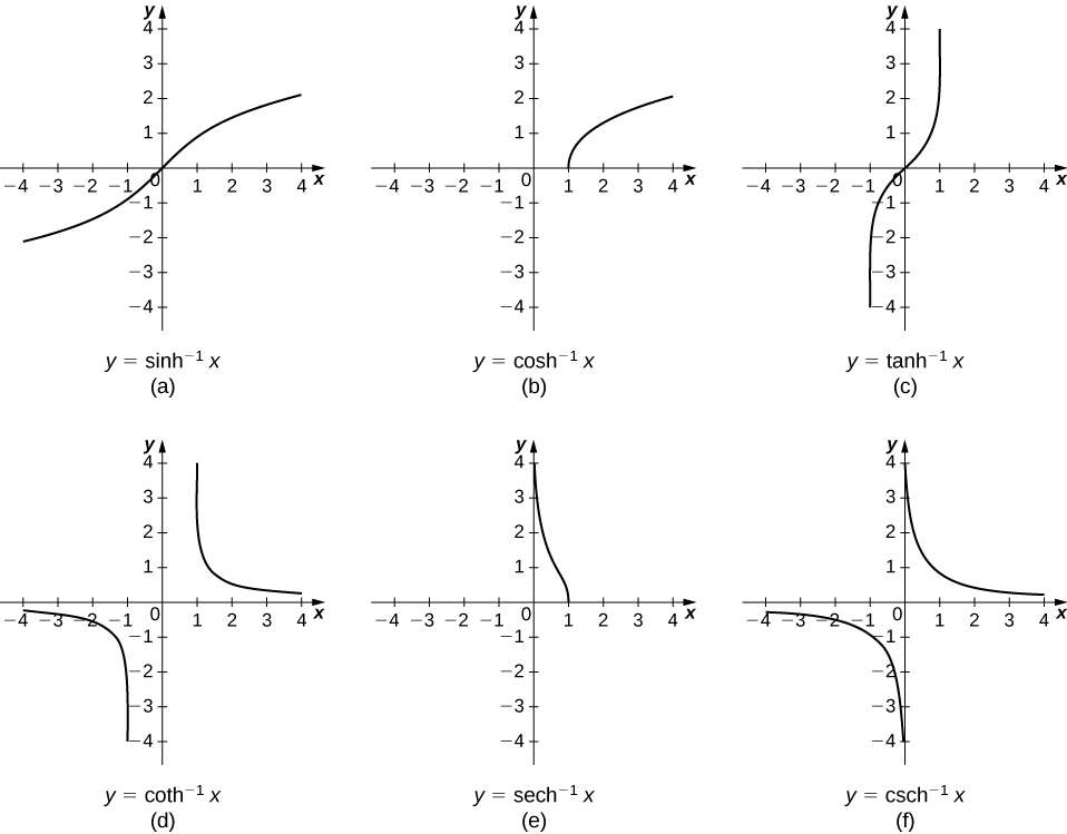
The graphs of the inverse hyperbolic functions are shown in the following figure.
To find the derivatives of the inverse functions, we use implicit differentiation. We have
Recall that [latex]{\text{cosh}}^{2}y-{\text{sinh}}^{2}y=1,[/latex] so [latex]\text{cosh}y=\sqrt{1+{\text{sinh}}^{2}y}.[/latex] Then,
We can derive differentiation formulas for the other inverse hyperbolic functions in a similar fashion. These differentiation formulas are summarized in the following table.
| [latex]f(x)[/latex] | [latex]\frac{d}{dx}f(x)[/latex] |
|---|---|
| [latex]{\text{sinh}}^{-1}x[/latex] | [latex]\frac{1}{\sqrt{1+{x}^{2}}}[/latex] |
| [latex]{\text{cosh}}^{-1}x[/latex] | [latex]\frac{1}{\sqrt{{x}^{2}-1}}[/latex] |
| [latex]{\text{tanh}}^{-1}x[/latex] | [latex]\frac{1}{1-{x}^{2}}[/latex] |
| [latex]{\text{coth}}^{-1}x[/latex] | [latex]\frac{1}{1-{x}^{2}}[/latex] |
| [latex]{\text{sech}}^{-1}x[/latex] | [latex]\frac{-1}{x\sqrt{1-{x}^{2}}}[/latex] |
| [latex]{\text{csch}}^{-1}x[/latex] | [latex]\frac{-1}{|x|\sqrt{1+{x}^{2}}}[/latex] |
Note that the derivatives of [latex]{\text{tanh}}^{-1}x[/latex] and [latex]{\text{coth}}^{-1}x[/latex] are the same. Thus, when we integrate [latex]1\text{/}(1-{x}^{2}),[/latex] we need to select the proper antiderivative based on the domain of the functions and the values of [latex]x.[/latex] Integration formulas involving the inverse hyperbolic functions are summarized as follows.
Differentiating Inverse Hyperbolic Functions
Evaluate the following derivatives:
- [latex]\frac{d}{dx}({\text{sinh}}^{-1}(\frac{x}{3}))[/latex]
- [latex]\frac{d}{dx}{({\text{tanh}}^{-1}x)}^{2}[/latex]
Evaluate the following derivatives:
- [latex]\frac{d}{dx}({\text{cosh}}^{-1}(3x))[/latex]
- [latex]\frac{d}{dx}{({\text{coth}}^{-1}x)}^{3}[/latex]
Hint
Use the formulas in (Figure) and apply the chain rule as necessary.
Integrals Involving Inverse Hyperbolic Functions
Evaluate the following integrals:
- [latex]\int \frac{1}{\sqrt{4{x}^{2}-1}}dx[/latex]
- [latex]\int \frac{1}{2x\sqrt{1-9{x}^{2}}}dx[/latex]
Evaluate the following integrals:
- [latex]\int \frac{1}{\sqrt{{x}^{2}-4}}dx,\text{}x>2[/latex]
- [latex]\int \frac{1}{\sqrt{1-{e}^{2x}}}dx[/latex]
Hint
Use the formulas above and apply [latex]u\text{-substitution}[/latex] as necessary.
Applications
One physical application of hyperbolic functions involves hanging cables. If a cable of uniform density is suspended between two supports without any load other than its own weight, the cable forms a curve called a catenary. High-voltage power lines, chains hanging between two posts, and strands of a spider’s web all form catenaries. The following figure shows chains hanging from a row of posts.
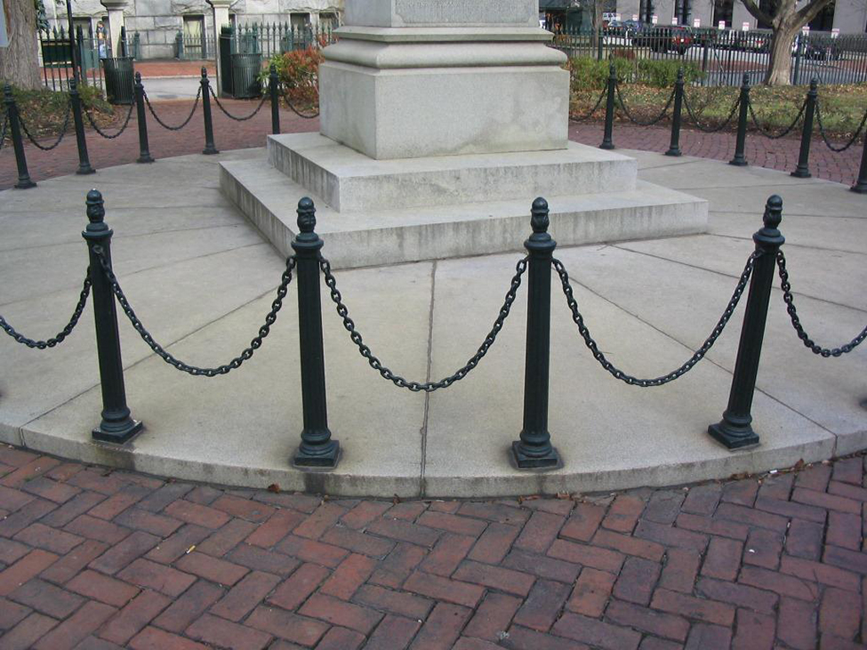
Figure 3. Chains between these posts take the shape of a catenary. (credit: modification of work by OKFoundryCompany, Flickr)
Hyperbolic functions can be used to model catenaries. Specifically, functions of the form [latex]y=a\text{cosh}(x\text{/}a)[/latex] are catenaries. (Figure) shows the graph of [latex]y=2\text{cosh}(x\text{/}2).[/latex]
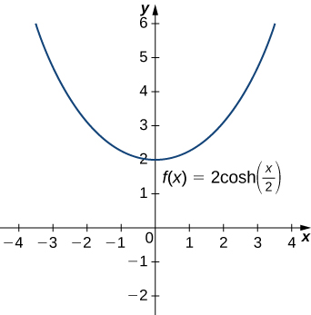
Figure 4. A hyperbolic cosine function forms the shape of a catenary.
Using a Catenary to Find the Length of a Cable
Assume a hanging cable has the shape [latex]10\text{cosh}(x\text{/}10)[/latex] for [latex]-15\le x\le 15,[/latex] where [latex]x[/latex] is measured in feet. Determine the length of the cable (in feet).
Assume a hanging cable has the shape [latex]15\text{cosh}(x\text{/}15)[/latex] for [latex]-20\le x\le 20.[/latex] Determine the length of the cable (in feet).
Hint
Use the procedure from the previous example.
Key Concepts
- Hyperbolic functions are defined in terms of exponential functions.
- Term-by-term differentiation yields differentiation formulas for the hyperbolic functions. These differentiation formulas give rise, in turn, to integration formulas.
- With appropriate range restrictions, the hyperbolic functions all have inverses.
- Implicit differentiation yields differentiation formulas for the inverse hyperbolic functions, which in turn give rise to integration formulas.
- The most common physical applications of hyperbolic functions are calculations involving catenaries.
1. [T] Find expressions for [latex]\text{cosh}x+\text{sinh}x[/latex] and [latex]\text{cosh}x-\text{sinh}x.[/latex] Use a calculator to graph these functions and ensure your expression is correct.
2. From the definitions of [latex]\text{cosh}(x)[/latex] and [latex]\text{sinh}(x),[/latex] find their antiderivatives.
3. Show that [latex]\text{cosh}(x)[/latex] and [latex]\text{sinh}(x)[/latex] satisfy [latex]y\text{″}=y.[/latex]
4. Use the quotient rule to verify that [latex]\text{tanh}(x)\prime ={\text{sech}}^{2}(x).[/latex]
5. Derive [latex]{\text{cosh}}^{2}(x)+{\text{sinh}}^{2}(x)=\text{cosh}(2x)[/latex] from the definition.
6. Take the derivative of the previous expression to find an expression for [latex]\text{sinh}(2x).[/latex]
7. Prove [latex]\text{sinh}(x+y)=\text{sinh}(x)\text{cosh}(y)+\text{cosh}(x)\text{sinh}(y)[/latex] by changing the expression to exponentials.
8. Take the derivative of the previous expression to find an expression for [latex]\text{cosh}(x+y).[/latex]
For the following exercises, find the derivatives of the given functions and graph along with the function to ensure your answer is correct.
9. [T][latex]\text{cosh}(3x+1)[/latex]
10. [T][latex]\text{sinh}({x}^{2})[/latex]
11. [T][latex]\frac{1}{\text{cosh}(x)}[/latex]
12. [T][latex]\text{sinh}(\text{ln}(x))[/latex]
13. [T][latex]{\text{cosh}}^{2}(x)+{\text{sinh}}^{2}(x)[/latex]
14. [T][latex]{\text{cosh}}^{2}(x)-{\text{sinh}}^{2}(x)[/latex]
15. [T][latex]\text{tanh}(\sqrt{{x}^{2}+1})[/latex]
16. [T][latex]\frac{1+\text{tanh}(x)}{1-\text{tanh}(x)}[/latex]
17. [T][latex]{\text{sinh}}^{6}(x)[/latex]
18. [T][latex]\text{ln}(\text{sech}(x)+\text{tanh}(x))[/latex]
For the following exercises, find the antiderivatives for the given functions.
19. [latex]\text{cosh}(2x+1)[/latex]
20. [latex]\text{tanh}(3x+2)[/latex]
21. [latex]x\text{cosh}({x}^{2})[/latex]
23. [latex]3{x}^{3}\text{tanh}({x}^{4})[/latex]
24. [latex]{\text{cosh}}^{2}(x)\text{sinh}(x)[/latex]
25. [latex]{\text{tanh}}^{2}(x){\text{sech}}^{2}(x)[/latex]
26. [latex]\frac{\text{sinh}(x)}{1+\text{cosh}(x)}[/latex]
27. [latex]\text{coth}(x)[/latex]
28. [latex]\text{cosh}(x)+\text{sinh}(x)[/latex]
29. [latex]{(\text{cosh}(x)+\text{sinh}(x))}^{n}[/latex]
For the following exercises, find the derivatives for the functions.
30. [latex]{\text{tanh}}^{-1}(4x)[/latex]
31. [latex]{\text{sinh}}^{-1}({x}^{2})[/latex]
32. [latex]{\text{sinh}}^{-1}(\text{cosh}(x))[/latex]
33. [latex]{\text{cosh}}^{-1}({x}^{3})[/latex]
34. [latex]{\text{tanh}}^{-1}( \cos (x))[/latex]
35. [latex]{e}^{{\text{sinh}}^{-1}(x)}[/latex]
36. [latex]\text{ln}({\text{tanh}}^{-1}(x))[/latex]
For the following exercises, find the antiderivatives for the functions.
37. [latex]\int \frac{dx}{4-{x}^{2}}[/latex]
38. [latex]\int \frac{dx}{{a}^{2}-{x}^{2}}[/latex]
39. [latex]\int \frac{dx}{\sqrt{{x}^{2}+1}}[/latex]
40. [latex]\int \frac{xdx}{\sqrt{{x}^{2}+1}}[/latex]
41. [latex]\int -\frac{dx}{x\sqrt{1-{x}^{2}}}[/latex]
42. [latex]\int \frac{{e}^{x}}{\sqrt{{e}^{2x}-1}}[/latex]
43. [latex]\int -\frac{2x}{{x}^{4}-1}[/latex]
For the following exercises, use the fact that a falling body with friction equal to velocity squared obeys the equation [latex]dv\text{/}dt=g-{v}^{2}.[/latex]
44. Show that [latex]v(t)=\sqrt{g}\text{tanh}(\sqrt{gt})[/latex] satisfies this equation.
45. Derive the previous expression for [latex]v(t)[/latex] by integrating [latex]\frac{dv}{g-{v}^{2}}=dt.[/latex]
46. [T] Estimate how far a body has fallen in 12 seconds by finding the area underneath the curve of [latex]v(t).[/latex]
For the following exercises, use this scenario: A cable hanging under its own weight has a slope [latex]S=dy\text{/}dx[/latex] that satisfies [latex]dS\text{/}dx=c\sqrt{1+{S}^{2}}.[/latex] The constant [latex]c[/latex] is the ratio of cable density to tension.
48. Show that [latex]S=\text{sinh}(cx)[/latex] satisfies this equation.
49. Integrate [latex]dy\text{/}dx=\text{sinh}(cx)[/latex] to find the cable height [latex]y(x)[/latex] if [latex]y(0)=1\text{/}c.[/latex]
50. Sketch the cable and determine how far down it sags at [latex]x=0.[/latex]
For the following exercises, solve each problem.
51. [T] A chain hangs from two posts 2 m apart to form a catenary described by the equation [latex]y=2\text{cosh}(x\text{/}2)-1.[/latex] Find the slope of the catenary at the left fence post.
52. [T] A chain hangs from two posts four meters apart to form a catenary described by the equation [latex]y=4\text{cosh}(x\text{/}4)-3.[/latex] Find the total length of the catenary (arc length).
53. [T] A high-voltage power line is a catenary described by [latex]y=10\text{cosh}(x\text{/}10).[/latex] Find the ratio of the area under the catenary to its arc length. What do you notice?
54. A telephone line is a catenary described by [latex]y=a\text{cosh}(x\text{/}a).[/latex] Find the ratio of the area under the catenary to its arc length. Does this confirm your answer for the previous question?
55. Prove the formula for the derivative of [latex]y={\text{sinh}}^{-1}(x)[/latex] by differentiating [latex]x=\text{sinh}(y).[/latex] (Hint: Use hyperbolic trigonometric identities.)
56. Prove the formula for the derivative of [latex]y={\text{cosh}}^{-1}(x)[/latex] by differentiating [latex]x=\text{cosh}(y).[/latex]
(Hint: Use hyperbolic trigonometric identities.)
57. Prove the formula for the derivative of [latex]y={\text{sech}}^{-1}(x)[/latex] by differentiating [latex]x=\text{sech}(y).[/latex] (Hint: Use hyperbolic trigonometric identities.)
58. Prove that [latex]{(\text{cosh}(x)+\text{sinh}(x))}^{n}=\text{cosh}(nx)+\text{sinh}(nx).[/latex]
59. Prove the expression for [latex]{\text{sinh}}^{-1}(x).[/latex] Multiply [latex]x=\text{sinh}(y)=(1\text{/}2)({e}^{y}-{e}^{\text{−}y})[/latex] by [latex]2{e}^{y}[/latex] and solve for [latex]y.[/latex] Does your expression match the textbook?
60. Prove the expression for [latex]{\text{cosh}}^{-1}(x).[/latex] Multiply [latex]x=\text{cosh}(y)=(1\text{/}2)({e}^{y}-{e}^{\text{−}y})[/latex] by [latex]2{e}^{y}[/latex] and solve for [latex]y.[/latex] Does your expression match the textbook?
Glossary
- catenary
- a curve in the shape of the function [latex]y=a\text{cosh}(x\text{/}a)[/latex] is a catenary; a cable of uniform density suspended between two supports assumes the shape of a catenary
Candela Citations
- Calculus I. Provided by: OpenStax. Located at: http://cnx.org/contents/8b89d172-2927-466f-8661-01abc7ccdba4@2.89. License: CC BY-NC-SA: Attribution-NonCommercial-ShareAlike. License Terms: Download for free at http://cnx.org/contents/8b89d172-2927-466f-8661-01abc7ccdba4@2.89

Hint
Use the formulas in (Figure) and apply the chain rule as necessary.