Learning Objectives
- Use the exponential growth model in applications, including population growth and compound interest.
- Explain the concept of doubling time.
- Use the exponential decay model in applications, including radioactive decay and Newton’s law of cooling.
- Explain the concept of half-life.
One of the most prevalent applications of exponential functions involves growth and decay models. Exponential growth and decay show up in a host of natural applications. From population growth and continuously compounded interest to radioactive decay and Newton’s law of cooling, exponential functions are ubiquitous in nature. In this section, we examine exponential growth and decay in the context of some of these applications.
Exponential Growth Model
Many systems exhibit exponential growth. These systems follow a model of the form [latex]y={y}_{0}{e}^{kt},[/latex] where [latex]{y}_{0}[/latex] represents the initial state of the system and [latex]k[/latex] is a positive constant, called the growth constant. Notice that in an exponential growth model, we have
That is, the rate of growth is proportional to the current function value. This is a key feature of exponential growth. (Figure) involves derivatives and is called a differential equation. We learn more about differential equations in Introduction to Differential Equations in the second volume of this text.
Rule: Exponential Growth Model
Systems that exhibit exponential growth increase according to the mathematical model
where [latex]{y}_{0}[/latex] represents the initial state of the system and [latex]k>0[/latex] is a constant, called the growth constant.
Population growth is a common example of exponential growth. Consider a population of bacteria, for instance. It seems plausible that the rate of population growth would be proportional to the size of the population. After all, the more bacteria there are to reproduce, the faster the population grows. (Figure) and (Figure) represent the growth of a population of bacteria with an initial population of 200 bacteria and a growth constant of 0.02. Notice that after only 2 hours [latex](120[/latex] minutes), the population is 10 times its original size!
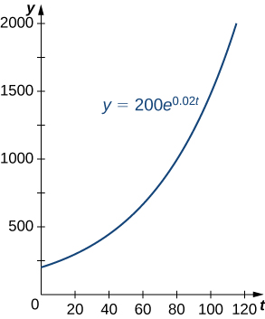
Figure 1. An example of exponential growth for bacteria.
| Time (min) | Population Size (no. of bacteria) |
|---|---|
| 10 | 244 |
| 20 | 298 |
| 30 | 364 |
| 40 | 445 |
| 50 | 544 |
| 60 | 664 |
| 70 | 811 |
| 80 | 991 |
| 90 | 1210 |
| 100 | 1478 |
| 110 | 1805 |
| 120 | 2205 |
Note that we are using a continuous function to model what is inherently discrete behavior. At any given time, the real-world population contains a whole number of bacteria, although the model takes on noninteger values. When using exponential growth models, we must always be careful to interpret the function values in the context of the phenomenon we are modeling.
Population Growth
Consider the population of bacteria described earlier. This population grows according to the function [latex]f(t)=200{e}^{0.02t},[/latex] where [latex]t[/latex] is measured in minutes. How many bacteria are present in the population after 5 hours [latex](300[/latex] minutes)? When does the population reach 100,000 bacteria?
Consider a population of bacteria that grows according to the function [latex]f(t)=500{e}^{0.05t},[/latex] where [latex]t[/latex] is measured in minutes. How many bacteria are present in the population after 4 hours? When does the population reach 100 million bacteria?
Let’s now turn our attention to a financial application: compound interest. Interest that is not compounded is called simple interest. Simple interest is paid once, at the end of the specified time period (usually 1 year). So, if we put [latex]$1000[/latex] in a savings account earning 2% simple interest per year, then at the end of the year we have
Compound interest is paid multiple times per year, depending on the compounding period. Therefore, if the bank compounds the interest every 6 months, it credits half of the year’s interest to the account after 6 months. During the second half of the year, the account earns interest not only on the initial [latex]$1000,[/latex] but also on the interest earned during the first half of the year. Mathematically speaking, at the end of the year, we have
Similarly, if the interest is compounded every 4 months, we have
and if the interest is compounded daily [latex](365[/latex] times per year), we have [latex]$1020.20.[/latex] If we extend this concept, so that the interest is compounded continuously, after [latex]t[/latex] years we have
Now let’s manipulate this expression so that we have an exponential growth function. Recall that the number [latex]e[/latex] can be expressed as a limit:
Based on this, we want the expression inside the parentheses to have the form [latex](1+1\text{/}m).[/latex] Let [latex]n=0.02m.[/latex] Note that as [latex]n\to \infty ,[/latex] [latex]m\to \infty[/latex] as well. Then we get
We recognize the limit inside the brackets as the number [latex]e.[/latex] So, the balance in our bank account after [latex]t[/latex] years is given by [latex]1000{e}^{0.02t}.[/latex] Generalizing this concept, we see that if a bank account with an initial balance of [latex]$P[/latex] earns interest at a rate of [latex]r\text{%},[/latex] compounded continuously, then the balance of the account after [latex]t[/latex] years is
Compound Interest
A 25-year-old student is offered an opportunity to invest some money in a retirement account that pays 5% annual interest compounded continuously. How much does the student need to invest today to have [latex]$1[/latex] million when she retires at age [latex]65?[/latex] What if she could earn 6% annual interest compounded continuously instead?
Suppose instead of investing at age [latex]25\sqrt{{b}^{2}-4ac},[/latex] the student waits until age 35. How much would she have to invest at [latex]5\text{%}?[/latex] At [latex]6\text{%}?[/latex]
Hint
Use the process from the previous example.
If a quantity grows exponentially, the time it takes for the quantity to double remains constant. In other words, it takes the same amount of time for a population of bacteria to grow from 100 to 200 bacteria as it does to grow from 10,000 to 20,000 bacteria. This time is called the doubling time. To calculate the doubling time, we want to know when the quantity reaches twice its original size. So we have
Definition
If a quantity grows exponentially, the doubling time is the amount of time it takes the quantity to double. It is given by
Using the Doubling Time
Assume a population of fish grows exponentially. A pond is stocked initially with 500 fish. After 6 months, there are 1000 fish in the pond. The owner will allow his friends and neighbors to fish on his pond after the fish population reaches 10,000. When will the owner’s friends be allowed to fish?
Suppose it takes 9 months for the fish population in (Figure) to reach 1000 fish. Under these circumstances, how long do the owner’s friends have to wait?
Hint
Use the process from the previous example.
Exponential Decay Model
Exponential functions can also be used to model populations that shrink (from disease, for example), or chemical compounds that break down over time. We say that such systems exhibit exponential decay, rather than exponential growth. The model is nearly the same, except there is a negative sign in the exponent. Thus, for some positive constant [latex]k,[/latex] we have [latex]y={y}_{0}{e}^{\text{−}kt}.[/latex]
As with exponential growth, there is a differential equation associated with exponential decay. We have
Rule: Exponential Decay Model
Systems that exhibit exponential decay behave according to the model
where [latex]{y}_{0}[/latex] represents the initial state of the system and [latex]k>0[/latex] is a constant, called the decay constant.
The following figure shows a graph of a representative exponential decay function.
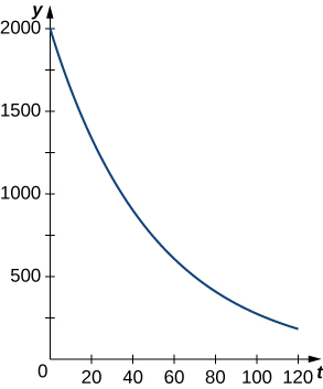
Figure 2. An example of exponential decay.
Let’s look at a physical application of exponential decay. Newton’s law of cooling says that an object cools at a rate proportional to the difference between the temperature of the object and the temperature of the surroundings. In other words, if [latex]T[/latex] represents the temperature of the object and [latex]{T}_{a}[/latex] represents the ambient temperature in a room, then
Note that this is not quite the right model for exponential decay. We want the derivative to be proportional to the function, and this expression has the additional [latex]{T}_{a}[/latex] term. Fortunately, we can make a change of variables that resolves this issue. Let [latex]y(t)=T(t)-{T}_{a}.[/latex] Then [latex]{y}^{\prime }(t)={T}^{\prime }(t)-0={T}^{\prime }(t),[/latex] and our equation becomes
From our previous work, we know this relationship between [latex]y[/latex] and its derivative leads to exponential decay. Thus,
and we see that
where [latex]{T}_{0}[/latex] represents the initial temperature. Let’s apply this formula in the following example.
Newton’s Law of Cooling
According to experienced baristas, the optimal temperature to serve coffee is between [latex]155\text{°}\text{F}[/latex] and [latex]175\text{°}\text{F}.[/latex] Suppose coffee is poured at a temperature of [latex]200\text{°}\text{F},[/latex] and after 2 minutes in a [latex]70\text{°}\text{F}[/latex] room it has cooled to [latex]180\text{°}\text{F}.[/latex] When is the coffee first cool enough to serve? When is the coffee too cold to serve? Round answers to the nearest half minute.
Suppose the room is warmer [latex](75\text{°}\text{F})[/latex] and, after 2 minutes, the coffee has cooled only to [latex]185\text{°}\text{F}.[/latex] When is the coffee first cool enough to serve? When is the coffee be too cold to serve? Round answers to the nearest half minute.
Hint
Use the process from the previous example.
Just as systems exhibiting exponential growth have a constant doubling time, systems exhibiting exponential decay have a constant half-life. To calculate the half-life, we want to know when the quantity reaches half its original size. Therefore, we have
Note: This is the same expression we came up with for doubling time.
Definition
If a quantity decays exponentially, the half-life is the amount of time it takes the quantity to be reduced by half. It is given by
Radiocarbon Dating
One of the most common applications of an exponential decay model is carbon dating. [latex]\text{Carbon-}14[/latex] decays (emits a radioactive particle) at a regular and consistent exponential rate. Therefore, if we know how much carbon was originally present in an object and how much carbon remains, we can determine the age of the object. The half-life of [latex]\text{carbon-}14[/latex] is approximately 5730 years—meaning, after that many years, half the material has converted from the original [latex]\text{carbon-}14[/latex] to the new nonradioactive [latex]\text{nitrogen-}14.[/latex] If we have 100 g [latex]\text{carbon-}14[/latex] today, how much is left in 50 years? If an artifact that originally contained 100 g of carbon now contains 10 g of carbon, how old is it? Round the answer to the nearest hundred years.
If we have 100 g of [latex]\text{carbon-}14,[/latex] how much is left after. years? If an artifact that originally contained 100 g of carbon now contains [latex]20g[/latex] of carbon, how old is it? Round the answer to the nearest hundred years.
Hint
Use the process from the previous example.
Key Concepts
- Exponential growth and exponential decay are two of the most common applications of exponential functions.
- Systems that exhibit exponential growth follow a model of the form [latex]y={y}_{0}{e}^{kt}.[/latex]
- In exponential growth, the rate of growth is proportional to the quantity present. In other words, [latex]{y}^{\prime }=ky.[/latex]
- Systems that exhibit exponential growth have a constant doubling time, which is given by [latex](\text{ln}2)\text{/}k.[/latex]
- Systems that exhibit exponential decay follow a model of the form [latex]y={y}_{0}{e}^{\text{−}kt}.[/latex]
- Systems that exhibit exponential decay have a constant half-life, which is given by [latex](\text{ln}2)\text{/}k.[/latex]
True or False? If true, prove it. If false, find the true answer.
1. The doubling time for [latex]y={e}^{ct}[/latex] is [latex](\text{ln}(2))\text{/}(\text{ln}(c)).[/latex]
2. If you invest [latex]$500,[/latex] an annual rate of interest of 3% yields more money in the first year than a 2.5% continuous rate of interest.
3. If you leave a [latex]100\text{°}\text{C}[/latex] pot of tea at room temperature [latex](25\text{°}\text{C})[/latex] and an identical pot in the refrigerator [latex](5\text{°}\text{C}),[/latex] with [latex]k=0.02,[/latex] the tea in the refrigerator reaches a drinkable temperature [latex](70\text{°}\text{C})[/latex] more than 5 minutes before the tea at room temperature.
4. If given a half-life of [latex]t[/latex] years, the constant [latex]k[/latex] for [latex]y={e}^{kt}[/latex] is calculated by [latex]k=\text{ln}(1\text{/}2)\text{/}t.[/latex]
False; [latex]k=\frac{\text{ln}(2)}{t}[/latex]
For the following exercises, use [latex]y={y}_{0}{e}^{kt}.[/latex]
5. If a culture of bacteria doubles in 3 hours, how many hours does it take to multiply by [latex]10?[/latex]
6. If bacteria increase by a factor of 10 in 10 hours, how many hours does it take to increase by [latex]100?[/latex]
7. How old is a skull that contains one-fifth as much radiocarbon as a modern skull? Note that the half-life of radiocarbon is 5730 years.
8. If a relic contains 90% as much radiocarbon as new material, can it have come from the time of Christ (approximately 2000 years ago)? Note that the half-life of radiocarbon is 5730 years.
9. The population of Cairo grew from 5 million to 10 million in 20 years. Use an exponential model to find when the population was 8 million.
10. The populations of New York and Los Angeles are growing at 1% and 1.4% a year, respectively. Starting from 8 million (New York) and 6 million (Los Angeles), when are the populations equal?
11. Suppose the value of [latex]$1[/latex] in Japanese yen decreases at 2% per year. Starting from [latex]$1=\text{¥}250,[/latex] when will [latex]$1=\text{¥}1?[/latex]
12. The effect of advertising decays exponentially. If 40% of the population remembers a new product after 3 days, how long will 20% remember it?
13. If [latex]y=1000[/latex] at [latex]t=3[/latex] and [latex]y=3000[/latex] at [latex]t=4,[/latex] what was [latex]{y}_{0}[/latex] at [latex]t=0?[/latex]
14. If [latex]y=100[/latex] at [latex]t=4[/latex] and [latex]y=10[/latex] at [latex]t=8,[/latex] when does [latex]y=1?[/latex]
15. If a bank offers annual interest of 7.5% or continuous interest of [latex]7.25\text{%},[/latex] which has a better annual yield?
16. What continuous interest rate has the same yield as an annual rate of [latex]9\text{%}?[/latex]
17. If you deposit [latex]$5000[/latex] at 8% annual interest, how many years can you withdraw [latex]$500[/latex] (starting after the first year) without running out of money?
18. You are trying to save [latex]$50,000[/latex] in 20 years for college tuition for your child. If interest is a continuous [latex]10\text{%},[/latex] how much do you need to invest initially?
19. You are cooling a turkey that was taken out of the oven with an internal temperature of [latex]165\text{°}\text{F}.[/latex] After 10 minutes of resting the turkey in a [latex]70\text{°}\text{F}[/latex] apartment, the temperature has reached [latex]155\text{°}\text{F}\text{.}[/latex] What is the temperature of the turkey 20 minutes after taking it out of the oven?
20. You are trying to thaw some vegetables that are at a temperature of [latex]1\text{°}\text{F}\text{.}[/latex] To thaw vegetables safely, you must put them in the refrigerator, which has an ambient temperature of [latex]44\text{°}\text{F}.[/latex] You check on your vegetables 2 hours after putting them in the refrigerator to find that they are now [latex]12\text{°}\text{F}\text{.}[/latex] Plot the resulting temperature curve and use it to determine when the vegetables reach [latex]33\text{°}\text{F}\text{.}[/latex]
21. You are an archaeologist and are given a bone that is claimed to be from a Tyrannosaurus Rex. You know these dinosaurs lived during the Cretaceous Era [latex](146[/latex] million years to 65 million years ago), and you find by radiocarbon dating that there is 0.000001% the amount of radiocarbon. Is this bone from the Cretaceous?
22. The spent fuel of a nuclear reactor contains plutonium-239, which has a half-life of 24,000 years. If 1 barrel containing 10kg of plutonium-239 is sealed, how many years must pass until only [latex]10g[/latex] of plutonium-239 is left?
For the next set of exercises, use the following table, which features the world population by decade.
| Years since 1950 | Population (millions) |
|---|---|
| 0 | 2,556 |
| 10 | 3,039 |
| 20 | 3,706 |
| 30 | 4,453 |
| 40 | 5,279 |
| 50 | 6,083 |
| 60 | 6,849 |
23. [T] The best-fit exponential curve to the data of the form [latex]P(t)=a{e}^{bt}[/latex] is given by [latex]P(t)=2686{e}^{0.01604t}.[/latex] Use a graphing calculator to graph the data and the exponential curve together.
24. [T] Find and graph the derivative [latex]{y}^{\prime }[/latex] of your equation. Where is it increasing and what is the meaning of this increase?
25. [T] Find and graph the second derivative of your equation. Where is it increasing and what is the meaning of this increase?
26. [T] Find the predicted date when the population reaches 10 billion. Using your previous answers about the first and second derivatives, explain why exponential growth is unsuccessful in predicting the future.
For the next set of exercises, use the following table, which shows the population of San Francisco during the 19th century.
| Years since 1850 | Population (thousands) |
|---|---|
| 0 | 21.00 |
| 10 | 56.80 |
| 20 | 149.5 |
| 30 | 234.0 |
27. [T] The best-fit exponential curve to the data of the form [latex]P(t)=a{e}^{bt}[/latex] is given by [latex]P(t)=35.26{e}^{0.06407t}.[/latex] Use a graphing calculator to graph the data and the exponential curve together.
28. [T] Find and graph the derivative [latex]{y}^{\prime }[/latex] of your equation. Where is it increasing? What is the meaning of this increase? Is there a value where the increase is maximal?
29. [T] Find and graph the second derivative of your equation. Where is it increasing? What is the meaning of this increase?
Glossary
- doubling time
- if a quantity grows exponentially, the doubling time is the amount of time it takes the quantity to double, and is given by [latex](\text{ln}2)\text{/}k[/latex]
- exponential decay
- systems that exhibit exponential decay follow a model of the form [latex]y={y}_{0}{e}^{\text{−}kt}[/latex]
- exponential growth
- systems that exhibit exponential growth follow a model of the form [latex]y={y}_{0}{e}^{kt}[/latex]
- half-life
- if a quantity decays exponentially, the half-life is the amount of time it takes the quantity to be reduced by half. It is given by [latex](\text{ln}2)\text{/}k[/latex]
Candela Citations
- Calculus I. Provided by: OpenStax. Located at: http://cnx.org/contents/8b89d172-2927-466f-8661-01abc7ccdba4@2.89. License: CC BY-NC-SA: Attribution-NonCommercial-ShareAlike. License Terms: Download for free at http://cnx.org/contents/8b89d172-2927-466f-8661-01abc7ccdba4@2.89

Hint
Use the process from the previous example.