Learning Objectives

Integrate functions involving exponential functions.
Integrate functions involving logarithmic functions.

Exponential and logarithmic functions are used to model population growth, cell growth, and financial growth, as well as depreciation, radioactive decay, and resource consumption, to name only a few applications. In this section, we explore integration involving exponential and logarithmic functions.

Integrals of Exponential Functions

The exponential function is perhaps the most efficient function in terms of the operations of calculus. The exponential function, $y={e}^{x},$ is its own derivative and its own integral.

Rule: Integrals of Exponential Functions

Exponential functions can be integrated using the following formulas.

$\begin{array}{ccc}\int {e}^{x}dx\hfill & =\hfill & {e}^{x}+C\hfill \\ \int {a}^{x}dx\hfill & =\hfill & \frac{{a}^{x}}{\text{ln}a}+C\hfill \end{array}$

Finding an Antiderivative of an Exponential Function

Find the antiderivative of the exponential function $e$ ^{− $x$}.

Show Solution

Use substitution, setting $u=\text{−}x,$ and then $du=-1dx.$ Multiply the du equation by −1, so you now have $\text{−}du=dx.$ Then,

$\begin{array}{cc}\int {e}^{\text{−}x}dx\hfill & =\text{−}\int {e}^{u}du\hfill \\ \\ & =\text{−}{e}^{u}+C\hfill \\ & =\text{−}{e}^{\text{−}x}+C.\hfill \end{array}$

Find the antiderivative of the function using substitution: ${x}^{2}{e}^{-2{x}^{3}}.$

Show Solution

$\int {x}^{2}{e}^{-2{x}^{3}}dx=-\frac{1}{6}{e}^{-2{x}^{3}}+C$

Hint

Let $u$ equal the exponent on $e$ .

A common mistake when dealing with exponential expressions is treating the exponent on $e$ the same way we treat exponents in polynomial expressions. We cannot use the power rule for the exponent on $e$ . This can be especially confusing when we have both exponentials and polynomials in the same expression, as in the previous checkpoint. In these cases, we should always double-check to make sure we’re using the right rules for the functions we’re integrating.

Square Root of an Exponential Function

Find the antiderivative of the exponential function ${e}^{x}\sqrt{1+{e}^{x}}.$

Show Solution

First rewrite the problem using a rational exponent:

$\int {e}^{x}\sqrt{1+{e}^{x}}dx=\int {e}^{x}{(1+{e}^{x})}^{1\text{/}2}dx.$

Using substitution, choose $u=1+{e}^{x}.u=1+{e}^{x}.$ Then, $du={e}^{x}dx.$ We have ((Figure))

$\int {e}^{x}{(1+{e}^{x})}^{1\text{/}2}dx=\int {u}^{1\text{/}2}du.$

Then

$\int {u}^{1\text{/}2}du=\frac{{u}^{3\text{/}2}}{3\text{/}2}+C=\frac{2}{3}{u}^{3\text{/}2}+C=\frac{2}{3}{(1+{e}^{x})}^{3\text{/}2}+C.$

A graph of the function f(x) = e^x * sqrt(1 + e^x), which is an increasing concave up curve, over [-3, 1]. It begins close to the x axis in quadrant two, crosses the y axis at (0, sqrt(2)), and continues to increase rapidly.

Figure 1. The graph shows an exponential function times the square root of an exponential function.

Find the antiderivative of ${e}^{x}{(3{e}^{x}-2)}^{2}.$

$\int {e}^{x}{(3{e}^{x}-2)}^{2}dx=\frac{1}{9}{(3{e}^{x}-2)}^{3}$

Hint

Let $u=3{e}^{x}-2u=3{e}^{x}-2.$

Using Substitution with an Exponential Function

Use substitution to evaluate the indefinite integral

$\int 3{x}^{2}{e}^{2{x}^{3}}dx.$

Show Solution

Here we choose to let $u$ equal the expression in the exponent on $e$ . Let $u=2{x}^{3}$ and $du=6{x}^{2}dx..$ Again, du is off by a constant multiplier; the original function contains a factor of 3 $x$ ², not 6 $x$ ². Multiply both sides of the equation by $\frac{1}{2}$ so that the integrand in $u$ equals the integrand in $x$ . Thus,

$\int 3{x}^{2}{e}^{2{x}^{3}}dx=\frac{1}{2}\int {e}^{u}du.$

Integrate the expression in $u$ and then substitute the original expression in $x$ back into the $u$ integral:

$\frac{1}{2}\int {e}^{u}du=\frac{1}{2}{e}^{u}+C=\frac{1}{2}{e}^{2{x}^{3}}+C.$

Evaluate the indefinite integral $\int 2{x}^{3}{e}^{{x}^{4}}dx.$

Show Solution

$\int 2{x}^{3}{e}^{{x}^{4}}dx=\frac{1}{2}{e}^{{x}^{4}}$

Hint

Let $u={x}^{4}.$

As mentioned at the beginning of this section, exponential functions are used in many real-life applications. The number $e$ is often associated with compounded or accelerating growth, as we have seen in earlier sections about the derivative. Although the derivative represents a rate of change or a growth rate, the integral represents the total change or the total growth. Let’s look at an example in which integration of an exponential function solves a common business application.

A price–demand function tells us the relationship between the quantity of a product demanded and the price of the product. In general, price decreases as quantity demanded increases. The marginal price–demand function is the derivative of the price–demand function and it tells us how fast the price changes at a given level of production. These functions are used in business to determine the price–elasticity of demand, and to help companies determine whether changing production levels would be profitable.

Finding a Price–Demand Equation

Find the price–demand equation for a particular brand of toothpaste at a supermarket chain when the demand is 50 tubes per week at $2.35 per tube, given that the marginal price—demand function, ${p}^{\prime }(x),$ for $x$ number of tubes per week, is given as

$p\text{'}(x)=-0.015{e}^{-0.01x}.$

If the supermarket chain sells 100 tubes per week, what price should it set?

Show Solution

To find the price–demand equation, integrate the marginal price–demand function. First find the antiderivative, then look at the particulars. Thus,

$\begin{array}{}\\ \\ p(x)\hfill & =\int -0.015{e}^{-0.01x}dx\hfill \\ & =-0.015\int {e}^{-0.01x}dx.\hfill \end{array}$

Using substitution, let $u=-0.01x$ and $du=-0.01dx.$ Then, divide both sides of the du equation by −0.01. This gives

$\begin{array}{cc}\frac{-0.015}{-0.01}\int {e}^{u}du\hfill & =1.5\int {e}^{u}du\hfill \\ \\ & =1.5{e}^{u}+C\hfill \\ & =1.5{e}^{-0.01x}+C.\hfill \end{array}$

The next step is to solve for C. We know that when the price is $2.35 per tube, the demand is 50 tubes per week. This means

$\begin{array}{}\\ \\ p(50)\hfill & =1.5{e}^{-0.01(50)}+C\hfill \\ & =2.35.\hfill \end{array}$

Now, just solve for C:

$\begin{array}{}\\ C\hfill & =2.35-1.5{e}^{-0.5}\hfill \\ & =2.35-0.91\hfill \\ & =1.44.\hfill \end{array}$

Thus,

$p(x)=1.5{e}^{-0.01x}+1.44.$

If the supermarket sells 100 tubes of toothpaste per week, the price would be

$p(100)=1.5{e}^{-0.01(100)}+1.44=1.5{e}^{-1}+1.44\approx 1.99.$

The supermarket should charge $1.99 per tube if it is selling 100 tubes per week.

Evaluating a Definite Integral Involving an Exponential Function

Evaluate the definite integral ${\int }_{1}^{2}{e}^{1-x}dx.$

Show Solution

Again, substitution is the method to use. Let $u=1-x,$ so $du=-1dx$ or $\text{−}du=dx.$ Then $\int {e}^{1-x}dx=\text{−}\int {e}^{u}du.$ Next, change the limits of integration. Using the equation $u=1-x,$ we have

$\begin{array}{c}u=1-(1)=0\hfill \\ u=1-(2)=-1.\hfill \end{array}$

The integral then becomes

$\begin{array}{cc}{\int }_{1}^{2}{e}^{1-x}dx\hfill & =\text{−}{\int }_{0}^{-1}{e}^{u}du\hfill \\ \\ \\ & ={\int }_{-1}^{0}{e}^{u}du\hfill \\ & ={{e}^{u}|}_{-1}^{0}\hfill \\ & ={e}^{0}-({e}^{-1})\hfill \\ & =\text{−}{e}^{-1}+1.\hfill \end{array}$

See (Figure).

A graph of the function f(x) = e^(1-x) over [0, 3]. It crosses the y axis at (0, e) as a decreasing concave up curve and symptotically approaches 0 as x goes to infinity.

Figure 2. The indicated area can be calculated by evaluating a definite integral using substitution.

Evaluate ${\int }_{0}^{2}{e}^{2x}dx.$

Show Solution

$\frac{1}{2}{\int }_{0}^{4}{e}^{u}du=\frac{1}{2}({e}^{4}-1)$

Hint

Let $u=2x.$

Growth of Bacteria in a Culture

Suppose the rate of in a Petri dish is given by $q(t)={3}^{t},$ where $t$ is given in hours and $q(t)$ is given in thousands of bacteria per hour. If a culture starts with 10,000 bacteria, find a function $Q(t)$ that gives the number of bacteria in the Petri dish at any time $t$ . How many bacteria are in the dish after 2 hours?

Show Solution

We have

$Q(t)=\int {3}^{t}dt=\frac{{3}^{t}}{\text{ln}3}+C.$

Then, at $t=0$ we have $Q(0)=10=\frac{1}{\text{ln}3}+C,$ so $C\approx 9.090$ and we get

$Q(t)=\frac{{3}^{t}}{\text{ln}3}+9.090.$

At time $t=2,$ we have

$Q(2)=\frac{{3}^{2}}{\text{ln}3}+9.090$

$=17.282.$

After 2 hours, there are 17,282 bacteria in the dish.

From (Figure), suppose the bacteria grow at a rate of $q(t)={2}^{t}.$ Assume the culture still starts with 10,000 bacteria. Find $Q(t).$ How many bacteria are in the dish after 3 hours?

Show Solution

$Q(t)=\frac{{2}^{t}}{\text{ln}2}+8.557.$ There are 20,099 bacteria in the dish after 3 hours.

Hint

Use the procedure from (Figure) to solve the problem.

Fruit Fly Population Growth

Suppose a population of increases at a rate of $g(t)=2{e}^{0.02t},$ in flies per day. If the initial population of fruit flies is 100 flies, how many flies are in the population after 10 days?

Show Solution

Let $G(t)$ represent the number of flies in the population at time $t$ . Applying the net change theorem, we have

$\begin{array}{}\\ \\ G(10)\hfill & =G(0)+{\int }_{0}^{10}2{e}^{0.02t}dt\hfill \\ & =100+{\left[\frac{2}{0.02}{e}^{0.02t}\right]|}_{0}^{10}\hfill \\ & =100+{\left[100{e}^{0.02t}\right]|}_{0}^{10}\hfill \\ & =100+100{e}^{0.2}-100\hfill \\ & \approx 122.\hfill \end{array}$

There are 122 flies in the population after 10 days.

Suppose the rate of growth of the fly population is given by $g(t)={e}^{0.01t},$ and the initial fly population is 100 flies. How many flies are in the population after 15 days?

Show Solution

Hint

Use the process from (Figure) to solve the problem.

Evaluating a Definite Integral Using Substitution

Evaluate the definite integral using substitution: ${\int }_{1}^{2}\frac{{e}^{1\text{/}x}}{{x}^{2}}dx.$

Show Solution

This problem requires some rewriting to simplify applying the properties. First, rewrite the exponent on $e$ as a power of $x$ , then bring the $x$ ² in the denominator up to the numerator using a negative exponent. We have

${\int }_{1}^{2}\frac{{e}^{1\text{/}x}}{{x}^{2}}dx={\int }_{1}^{2}{e}^{{x}^{-1}}{x}^{-2}dx.$

Let $u={x}^{-1},$ the exponent on $e$ . Then

$\begin{array}{cc}\hfill du& =\text{−}{x}^{-2}dx\hfill \\ \hfill -du& ={x}^{-2}dx.\hfill \end{array}$

Bringing the negative sign outside the integral sign, the problem now reads

$\text{−}\int {e}^{u}du.$

Next, change the limits of integration:

$\begin{array}{}\\ \\ u={(1)}^{-1}=1\hfill \\ u={(2)}^{-1}=\frac{1}{2}.\hfill \end{array}$

Notice that now the limits begin with the larger number, meaning we must multiply by −1 and interchange the limits. Thus,

$\begin{array}{}\\ \\ \\ \text{−}{\int }_{1}^{1\text{/}2}{e}^{u}du\hfill & ={\int }_{1\text{/}2}^{1}{e}^{u}du\hfill \\ & ={e}^{u}{|}_{1\text{/}2}^{1}\hfill \\ & =e-{e}^{1\text{/}2}\hfill \\ & =e-\sqrt{e}.\hfill \end{array}$

Evaluate the definite integral using substitution: ${\int }_{1}^{2}\frac{1}{{x}^{3}}{e}^{4{x}^{-2}}dx.$

Show Solution

${\int }_{1}^{2}\frac{1}{{x}^{3}}{e}^{4{x}^{-2}}dx=\frac{1}{8}\left[{e}^{4}-e\right]$

Hint

Let $u=4{x}^{-2}.$

Integrals Involving Logarithmic Functions

Integrating functions of the form $f(x)={x}^{-1}$ result in the absolute value of the natural log function, as shown in the following rule. Integral formulas for other logarithmic functions, such as $f(x)=\text{ln}x$ and $f(x)={\text{log}}_{a}x,$ are also included in the rule.

Rule: Integration Formulas Involving Logarithmic Functions

The following formulas can be used to evaluate integrals involving logarithmic functions.

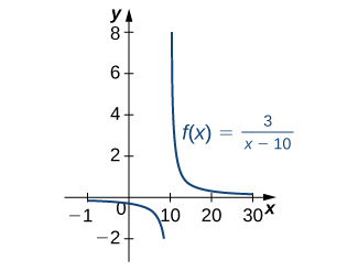
$\begin{array}{ccc}\hfill \int {x}^{-1}dx& =\hfill & \text{ln}|x|+C\hfill \\ \hfill \int \text{ln}xdx& =\hfill & x\text{ln}x-x+C=x(\text{ln}x-1)+C\hfill \\ \hfill \int {\text{log}}_{a}xdx& =\hfill & \frac{x}{\text{ln}a}(\text{ln}x-1)+C\hfill \end{array}$

Finding an Antiderivative Involving $\text{ln}x$

Find the antiderivative of the function $\frac{3}{x-10}.$

Show Solution

First factor the 3 outside the integral symbol. Then use the $u$ ⁻¹ rule. Thus,

$\begin{array}{ll}\int \frac{3}{x-10}dx\hfill & =3\int \frac{1}{x-10}dx\hfill \\ \\ \\ & =3\int \frac{du}{u}\hfill \\ & =3\text{ln}|u|+C\hfill \\ & =3\text{ln}|x-10|+C,x\ne 10.\hfill \end{array}$

See (Figure).

A graph of the function f(x) = 3 / (x – 10). There is an asymptote at x=10. The first segment is a decreasing concave down curve that approaches 0 as x goes to negative infinity and approaches negative infinity as x goes to 10. The second segment is a decreasing concave up curve that approaches infinity as x goes to 10 and approaches 0 as x approaches infinity.

Figure 3. The domain of this function is $x\ne 10.$

Find the antiderivative of $\frac{1}{x+2}.$

Show Solution

$\text{ln}|x+2|+C$

Hint

Follow the pattern from (Figure) to solve the problem.

Finding an Antiderivative of a Rational Function

Find the antiderivative of $\frac{2{x}^{3}+3x}{{x}^{4}+3{x}^{2}}.$

This can be rewritten as $\int (2{x}^{3}+3x){({x}^{4}+3{x}^{2})}^{-1}dx.$ Use substitution. Let $u={x}^{4}+3{x}^{2},$ then $du=4{x}^{3}+6x.$ Alter du by factoring out the 2. Thus,

$\begin{array}{}\\ \hfill du& =\hfill & (4{x}^{3}+6x)dx\hfill \\ & =\hfill & 2(2{x}^{3}+3x)dx\hfill \\ \hfill \frac{1}{2}du& =\hfill & (2{x}^{3}+3x)dx.\hfill \end{array}$

Rewrite the integrand in $u$ :

$\int (2{x}^{3}+3x){({x}^{4}+3{x}^{2})}^{-1}dx=\frac{1}{2}\int {u}^{-1}du.$

Then we have

$\begin{array}{ll}\frac{1}{2}\int {u}^{-1}du\hfill & =\frac{1}{2}\text{ln}|u|+C\hfill \\ \\ & =\frac{1}{2}\text{ln}|{x}^{4}+3{x}^{2}|+C.\hfill \end{array}$

Finding an Antiderivative of a Logarithmic Function

Find the antiderivative of the log function ${\text{log}}_{2}x.$

Show Solution

Follow the format in the formula listed in the rule on integration formulas involving logarithmic functions. Based on this format, we have

$\int {\text{log}}_{2}xdx=\frac{x}{\text{ln}2}(\text{ln}x-1)+C.$

Find the antiderivative of ${\text{log}}_{3}x.$

Show Solution

$\frac{x}{\text{ln}3}(\text{ln}x-1)+C$

Hint

Follow (Figure) and refer to the rule on integration formulas involving logarithmic functions.

(Figure) is a definite integral of a trigonometric function. With trigonometric functions, we often have to apply a trigonometric property or an identity before we can move forward. Finding the right form of the integrand is usually the key to a smooth integration.

Evaluating a Definite Integral

Find the definite integral of ${\int }_{0}^{\pi \text{/}2}\frac{ \sin x}{1+ \cos x}dx.$

Show Solution

We need substitution to evaluate this problem. Let $u=1+ \cos x,,$ so $du=\text{−} \sin xdx.$ Rewrite the integral in terms of $u$ , changing the limits of integration as well. Thus,

$\begin{array}{c}u=1+ \cos (0)=2\hfill \\ u=1+ \cos (\frac{\pi }{2})=1.\hfill \end{array}$

Then

$\begin{array}{cc}{\int }_{0}^{\pi \text{/}2}\frac{ \sin x}{1+ \cos x}\hfill & =\text{−}{\int }_{2}^{1}{u}^{-1}du\hfill \\ \\ \\ & ={\int }_{1}^{2}{u}^{-1}du\hfill \\ & ={\text{ln}|u||}_{1}^{2}\hfill \\ & =\left[\text{ln}2-\text{ln}1\right]\hfill \\ & =\text{ln}2.\hfill \end{array}$

Key Concepts

Exponential and logarithmic functions arise in many real-world applications, especially those involving growth and decay.
Substitution is often used to evaluate integrals involving exponential functions or logarithms.

Key Equations

Integrals of Exponential Functions
$\int {e}^{x}dx={e}^{x}+C$
$\int {a}^{x}dx=\frac{{a}^{x}}{\text{ln}a}+C$
Integration Formulas Involving Logarithmic Functions
$\int {x}^{-1}dx=\text{ln}|x|+C$
$\int \text{ln}xdx=x\text{ln}x-x+C=x(\text{ln}x-1)+C$
$\int {\text{log}}_{a}xdx=\frac{x}{\text{ln}a}(\text{ln}x-1)+C$

In the following exercises, compute each indefinite integral.

1. $\int {e}^{2x}dx$

2. $\int {e}^{-3x}dx$

Show Solution

$\frac{-1}{3}{e}^{-3x}+C$

3. $\int {2}^{x}dx$

4. $\int {3}^{\text{−}x}dx$

Show Solution

$-\frac{{3}^{\text{−}x}}{\text{ln}3}+C$

5. $\int \frac{1}{2x}dx$

6. $\int \frac{2}{x}dx$

Show Solution

$\text{ln}({x}^{2})+C$

7. $\int \frac{1}{{x}^{2}}dx$

8. $\int \frac{1}{\sqrt{x}}dx$

Show Solution

$2\sqrt{x}+C$

In the following exercises, find each indefinite integral by using appropriate substitutions.

9. $\int \frac{\text{ln}x}{x}dx$

10. $\int \frac{dx}{x{(\text{ln}x)}^{2}}$

Show Solution

$-\frac{1}{\text{ln}x}+C$

11. $\int \frac{dx}{x\text{ln}x}(x>1)$

12. $\int \frac{dx}{x\text{ln}x\text{ln}(\text{ln}x)}$

Show Solution

$\text{ln}(\text{ln}(\text{ln}x))+C$

13. $\int \tan \theta d\theta$

14. $\int \frac{ \cos x-x \sin x}{x \cos x}dx$

Show Solution

$\text{ln}(x \cos x)+C$

15. $\int \frac{\text{ln}( \sin x)}{ \tan x}dx$

16. $\int \text{ln}( \cos x) \tan xdx$

Show Solution

$-\frac{1}{2}{(\text{ln}( \cos (x)))}^{2}+C$

17. $\int x{e}^{\text{−}{x}^{2}}dx$

18. $\int {x}^{2}{e}^{\text{−}{x}^{3}}dx$

Show Solution

$\frac{\text{−}{e}^{\text{−}{x}^{3}}}{3}+C$

19. $\int {e}^{ \sin x} \cos xdx$

20. $\int {e}^{ \tan x}{ \sec }^{2}xdx$

Show Solution

${e}^{ \tan x}+C$

21. $\int {e}^{\text{ln}x}\frac{dx}{x}$

22. $\int \frac{{e}^{\text{ln}(1-t)}}{1-t}dt$

Show Solution

$t+C$

In the following exercises, verify by differentiation that $\int \text{ln}xdx=x(\text{ln}x-1)+C,$ then use appropriate changes of variables to compute the integral.

23. $\int \text{ln}xdx$ $(Hint\text{:}\int \text{ln}xdx=\frac{1}{2}\int x\text{ln}({x}^{2})dx)$

24. $\int {x}^{2}{\text{ln}}^{2}xdx$

Show Solution

$\frac{1}{9}{x}^{3}(\text{ln}({x}^{3})-1)+C$

25. $\int \frac{\text{ln}x}{{x}^{2}}dx$ $(Hint\text{:}\text{Set}u=\frac{1}{x}\text{.})$

26. $\int \frac{\text{ln}x}{\sqrt{x}}dx$ $(Hint\text{:}\text{Set}u=\sqrt{x}\text{.})$

Show Solution

$2\sqrt{x}(\text{ln}x-2)+C$

27. Write an integral to express the area under the graph of $y=\frac{1}{t}$ from $t=1$ to e^x and evaluate the integral.

28. Write an integral to express the area under the graph of $y={e}^{t}$ between $t=0$ and $t=\text{ln}x,$ and evaluate the integral.

Show Solution

${\int }_{0}^{\text{ln}x}{e}^{t}dt={e}^{t}{|}_{0}^{\text{ln}x}={e}^{\text{ln}x}-{e}^{0}=x-1$

In the following exercises, use appropriate substitutions to express the trigonometric integrals in terms of compositions with logarithms.

29. $\int \tan (2x)dx$

30. $\int \frac{ \sin (3x)- \cos (3x)}{ \sin (3x)+ \cos (3x)}dx$

Show Solution

$-\frac{1}{3}\text{ln}( \sin (3x)+ \cos (3x))$

31. $\int \frac{x \sin ({x}^{2})}{ \cos ({x}^{2})}dx$

32. $\int x \csc ({x}^{2})dx$

Show Solution

$-\frac{1}{2}\text{ln}| \csc ({x}^{2})+ \cot ({x}^{2})|+C$

33. $\int \text{ln}( \cos x) \tan xdx$

34. $\int \text{ln}( \csc x) \cot xdx$

Show Solution

$-\frac{1}{2}{(\text{ln}( \csc x))}^{2}+C$

35. $\int \frac{{e}^{x}-{e}^{\text{−}x}}{{e}^{x}+{e}^{\text{−}x}}dx$

In the following exercises, evaluate the definite integral.

36. ${\int }_{1}^{2}\frac{1+2x+{x}^{2}}{3x+3{x}^{2}+{x}^{3}}dx$

Show Solution

$\frac{1}{3}\text{ln}(\frac{26}{7})$

37. ${\int }_{0}^{\pi \text{/}4} \tan xdx$

38. ${\int }_{0}^{\pi \text{/}3}\frac{ \sin x- \cos x}{ \sin x+ \cos x}dx$

Show Solution

$\text{ln}(\sqrt{3}-1)$

39. ${\int }_{\pi \text{/}6}^{\pi \text{/}2} \csc xdx$

40. ${\int }_{\pi \text{/}4}^{\pi \text{/}3} \cot xdx$

Show Solution

$\frac{1}{2}\text{ln}\frac{3}{2}$

In the following exercises, integrate using the indicated substitution.

41. $\int \frac{x}{x-100}dx;u=x-100$

42. $\int \frac{y-1}{y+1}dy;u=y+1$

Show Solution

$y-2\text{ln}|y+1|+C$

43. $\int \frac{1-{x}^{2}}{3x-{x}^{3}}dx;u=3x-{x}^{3}$

44. $\int \frac{ \sin x+ \cos x}{ \sin x- \cos x}dx;u= \sin x- \cos x$

Show Solution

$\text{ln}| \sin x- \cos x|+C$

45. $\int {e}^{2x}\sqrt{1-{e}^{2x}}dx;u={e}^{2x}$

46. $\int \text{ln}(x)\frac{\sqrt{1-{(\text{ln}x)}^{2}}}{x}dx;u=\text{ln}x$

Show Solution

$-\frac{1}{3}{(1-(\text{ln}{x}^{2}))}^{3\text{/}2}+C$

In the following exercises, does the right-endpoint approximation overestimate or underestimate the exact area? Calculate the right endpoint estimate R₅₀ and solve for the exact area.

47. [T] $y={e}^{x}$ over $\left[0,1\right]$

48. [T] $y={e}^{\text{−}x}$ over $\left[0,1\right]$

Show Solution

Exact solution: $\frac{e-1}{e},{R}_{50}=0.6258.$ Since $f$ is decreasing, the right endpoint estimate underestimates the area.

49. [T] $y=\text{ln}(x)$ over $\left[1,2\right]$

50. [T] $y=\frac{x+1}{{x}^{2}+2x+6}$ over $\left[0,1\right]$

Show Solution

Exact solution: $\frac{2\text{ln}(3)-\text{ln}(6)}{2},{R}_{50}=0.2033.$ Since $f$ is increasing, the right endpoint estimate overestimates the area.

51. [T] $y={2}^{x}$ over $\left[-1,0\right]$

52. [T] $y=\text{−}{2}^{\text{−}x}$ over $\left[0,1\right]$

Show Solution

Exact solution: $-\frac{1}{\text{ln}(4)},{R}_{50}=-0.7164.$ Since $f$ is increasing, the right endpoint estimate overestimates the area (the actual area is a larger negative number).

In the following exercises, $f(x)\ge 0$ for $a\le x\le b.$ Find the area under the graph of $f(x)$ between the given values $a$ and $b$ by integrating.

53. $f(x)=\frac{{\text{log}}_{10}(x)}{x};a=10,b=100$

54. $f(x)=\frac{{\text{log}}_{2}(x)}{x};a=32,b=64$

Show Solution

$\frac{11}{2}\text{ln}2$

55. $f(x)={2}^{\text{−}x};a=1,b=2$

56. $f(x)={2}^{\text{−}x};a=3,b=4$

Show Solution

$\frac{1}{\text{ln}(65,536)}$

57. Find the area under the graph of the function $f(x)=x{e}^{\text{−}{x}^{2}}$ between $x=0$ and $x=5.$

58. Compute the integral of $f(x)=x{e}^{\text{−}{x}^{2}}$ and find the smallest value of N such that the area under the graph $f(x)=x{e}^{\text{−}{x}^{2}}$ between $x=N$ and $x=N+10$ is, at most, 0.01.

Show Solution

${\int }_{N}^{N+1}x{e}^{\text{−}{x}^{2}}dx=\frac{1}{2}({e}^{\text{−}{N}^{2}}-{e}^{\text{−}{(N+1)}^{2}}).$ The quantity is less than 0.01 when

$N=2.$

59. Find the limit, as N tends to infinity, of the area under the graph of $f(x)=x{e}^{\text{−}{x}^{2}}$ between $x=0$ and $x=5.$

60. Show that ${\int }_{a}^{b}\frac{dt}{t}={\int }_{1\text{/}b}^{1\text{/}a}\frac{dt}{t}$ when [latex]0

Show Solution

${\int }_{a}^{b}\frac{dx}{x}=\text{ln}(b)-\text{ln}(a)=\text{ln}(\frac{1}{a})-\text{ln}(\frac{1}{b})={\int }_{1\text{/}b}^{1\text{/}a}\frac{dx}{x}$

61. Suppose that $f(x)>0$ for all $x$ and that $f$ and $g$ are differentiable. Use the identity ${f}^{g}={e}^{g\text{ln}f}$ and the chain rule to find the derivative of ${f}^{g}.$

62. Use the previous exercise to find the antiderivative of $h(x)={x}^{x}(1+\text{ln}x)$ and evaluate ${\int }_{2}^{3}{x}^{x}(1+\text{ln}x)dx.$

Show Solution

63. Show that if $c>0,$ then the integral of $1\text{/}x$ from ac to bc [latex](0

The following exercises are intended to derive the fundamental properties of the natural log starting from the Definition/em> $\text{ln}(x)={\int }_{1}^{x}\frac{dt}{t},$ using properties of the definite integral and making no further assumptions.

64. Use the identity $\text{ln}(x)={\int }_{1}^{x}\frac{dt}{t}$ to derive the identity $\text{ln}(\frac{1}{x})=\text{−}\text{ln}x.$

Show Solution

We may assume that $x>1,\text{so}\frac{1}{x}<1.$ Then, ${\int }_{1}^{1\text{/}x}\frac{dt}{t}.$ Now make the substitution $u=\frac{1}{t},$ so $du=-\frac{dt}{{t}^{2}}$ and $\frac{du}{u}=-\frac{dt}{t},$ and change endpoints: ${\int }_{1}^{1\text{/}x}\frac{dt}{t}=\text{−}{\int }_{1}^{x}\frac{du}{u}=\text{−}\text{ln}x.$

65. Use a change of variable in the integral ${\int }_{1}^{xy}\frac{1}{t}dt$ to show that $\text{ln}xy=\text{ln}x+\text{ln}y\text{ for }x,y>0.$

66. Use the identity $\text{ln}x={\int }_{1}^{x}\frac{dt}{x}$ to show that $\text{ln}(x)$ is an increasing function of $x$ on $[0,\infty )$ and use the previous exercises to show that the range of $\text{ln}(x)$ is $(\text{−}\infty ,\infty ).$ Without any further assumptions, conclude that $\text{ln}(x)$ has an inverse function defined on $(\text{−}\infty ,\infty ).$

67. Pretend, for the moment, that we do not know that ${e}^{x}$ is the inverse function of $\text{ln}(x),$ but keep in mind that $\text{ln}(x)$ has an inverse function defined on $(\text{−}\infty ,\infty ).$ Call it E. Use the identity $\text{ln}xy=\text{ln}x+\text{ln}y$ to deduce that $E(a+b)=E(a)E(b)$ for any real numbers $a$ , $b$ .

68. Pretend, for the moment, that we do not know that ${e}^{x}$ is the inverse function of $\text{ln}x,$ but keep in mind that $\text{ln}x$ has an inverse function defined on $(\text{−}\infty ,\infty ).$ Call it E. Show that $E\text{'}(t)=E(t).$

Show Solution

$x=E(\text{ln}(x)).$ Then, $1=\frac{E\text{'}(\text{ln}x)}{x}\text{or}x=E\text{'}(\text{ln}x).$ Since any number $t$ can be written $t=\text{ln}x$ for some $x$ , and for such $t$ we have $x=E(t),$ it follows that for any $t,E\text{'}(t)=E(t).$

69. The sine integral, defined as $S(x)={\int }_{0}^{x}\frac{ \sin t}{t}dt$ is an important quantity in engineering. Although it does not have a simple closed formula, it is possible to estimate its behavior for large $x$ . Show that for $k\ge 1,|S(2\pi k)-S(2\pi (k+1))|\le \frac{1}{k(2k+1)\pi }.$ (Hint: $\sin (t+\pi )=\text{−} \sin t$ )

70. [T] The normal distribution in probability is given by $p(x)=\frac{1}{\sigma \sqrt{2\pi }}{e}^{\text{−}{(x-\mu )}^{2}\text{/}2{\sigma }^{2}},$ where σ is the standard deviation and μ is the average. The standard normal distribution in probability, ${p}_{s},$ corresponds to $\mu =0\text{ and }\sigma =1.$ Compute the left endpoint estimates ${R}_{10}\text{ and }{R}_{100}$ of ${\int }_{-1}^{1}\frac{1}{\sqrt{2\pi }}{e}^{\text{−}{x}^{2\text{/}2}}dx.$

Show Solution

${R}_{10}=0.6811,{R}_{100}=0.6827$

A graph of the function f(x) = .5 * ( sqrt(2)*e^(-.5x^2)) / sqrt(pi). It is a downward opening curve that is symmetric across the y axis, crossing at about (0, .4). It approaches 0 as x goes to positive and negative infinity. Between 1 and -1, ten rectangles are drawn for a right endpoint estimate of the area under the curve.

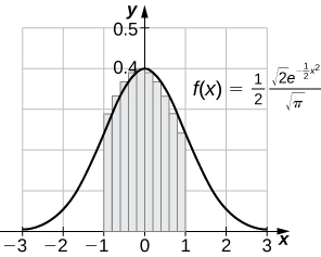
71. [T] Compute the right endpoint estimates ${R}_{50}\text{ and }{R}_{100}$ of ${\int }_{-3}^{5}\frac{1}{2\sqrt{2\pi }}{e}^{\text{−}{(x-1)}^{2}\text{/}8}.$

5. Integration

5.6 Integrals Involving Exponential and Logarithmic Functions

Learning Objectives

Integrals of Exponential Functions

Rule: Integrals of Exponential Functions

Finding an Antiderivative of an Exponential Function

Hint

Square Root of an Exponential Function

Hint

Using Substitution with an Exponential Function

Hint

Finding a Price–Demand Equation

Evaluating a Definite Integral Involving an Exponential Function

Hint

Growth of Bacteria in a Culture

Hint

Fruit Fly Population Growth

Hint

Evaluating a Definite Integral Using Substitution

Hint

Integrals Involving Logarithmic Functions

Rule: Integration Formulas Involving Logarithmic Functions

Finding an Antiderivative Involving $\text{ln}x$

Hint

Finding an Antiderivative of a Rational Function

Finding an Antiderivative of a Logarithmic Function

Hint

Evaluating a Definite Integral

Key Concepts

Key Equations

Candela Citations

5. Integration

5.6 Integrals Involving Exponential and Logarithmic Functions

Learning Objectives

Integrals of Exponential Functions

Rule: Integrals of Exponential Functions

Finding an Antiderivative of an Exponential Function

Hint

Square Root of an Exponential Function

Hint

Using Substitution with an Exponential Function

Hint

Finding a Price–Demand Equation

Evaluating a Definite Integral Involving an Exponential Function

Hint

Growth of Bacteria in a Culture

Hint

Fruit Fly Population Growth

Hint

Evaluating a Definite Integral Using Substitution

Hint

Integrals Involving Logarithmic Functions

Rule: Integration Formulas Involving Logarithmic Functions

Finding an Antiderivative Involving lnx\text{ln}x

Hint

Finding an Antiderivative of a Rational Function

Finding an Antiderivative of a Logarithmic Function

Hint

Evaluating a Definite Integral

Key Concepts

Key Equations

Finding an Antiderivative Involving $\text{ln}x$