Learning Objectives

Calculate the limit of a function as [latex]x[/latex] increases or decreases without bound.
Recognize a horizontal asymptote on the graph of a function.
Estimate the end behavior of a function as [latex]x[/latex] increases or decreases without bound.
Recognize an oblique asymptote on the graph of a function.
Analyze a function and its derivatives to draw its graph.

We have shown how to use the first and second derivatives of a function to describe the shape of a graph. To graph a function [latex]f[/latex] defined on an unbounded domain, we also need to know the behavior of [latex]f[/latex] as [latex]x \to \pm \infty[/latex]. In this section, we define limits at infinity and show how these limits affect the graph of a function. At the end of this section, we outline a strategy for graphing an arbitrary function [latex]f[/latex].

Limits at Infinity

We begin by examining what it means for a function to have a finite limit at infinity. Then we study the idea of a function with an infinite limit at infinity. Back in Introduction to Functions and Graphs, we looked at vertical asymptotes; in this section we deal with horizontal and oblique asymptotes.

Limits at Infinity and Horizontal Asymptotes

Recall that [latex]\underset{x \to a}{\lim}f(x)=L[/latex] means [latex]f(x)[/latex] becomes arbitrarily close to [latex]L[/latex] as long as [latex]x[/latex] is sufficiently close to [latex]a[/latex]. We can extend this idea to limits at infinity. For example, consider the function [latex]f(x)=2+\frac{1}{x}[/latex]. As can be seen graphically in (Figure) and numerically in (Figure), as the values of [latex]x[/latex] get larger, the values of [latex]f(x)[/latex] approach 2. We say the limit as [latex]x[/latex] approaches [latex]\infty [/latex] of [latex]f(x)[/latex] is 2 and write [latex]\underset{x\to \infty }{\lim}f(x)=2[/latex]. Similarly, for [latex]x<0[/latex], as the values [latex]|x|[/latex] get larger, the values of [latex]f(x)[/latex] approaches 2. We say the limit as [latex]x[/latex] approaches [latex]−\infty [/latex] of [latex]f(x)[/latex] is 2 and write [latex]\underset{x\to a}{\lim}f(x)=2[/latex].

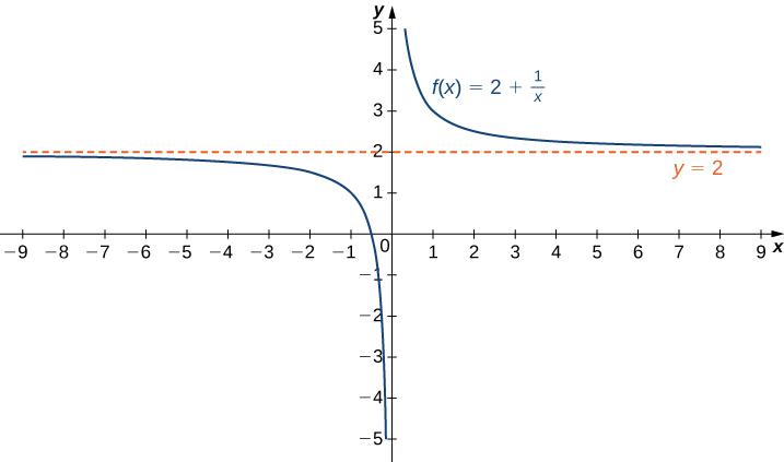
The function f(x) 2 + 1/x is graphed. The function starts negative near y = 2 but then decreases to −∞ near x = 0. The function then decreases from ∞ near x = 0 and gets nearer to y = 2 as x increases. There is a horizontal line denoting the asymptote y = 2.

Figure 1. The function approaches the asymptote [latex]y=2[/latex] as [latex]x[/latex] approaches [latex]\pm \infty[/latex].

Values of a function [latex]f[/latex] as [latex]x \to \pm \infty [/latex]
[latex]x[/latex]	10	100	1,000	10,000
[latex]2+\frac{1}{x}[/latex]	2.1	2.01	2.001	2.0001
[latex]x[/latex]	-10	-100	-1000	-10,000
[latex]2+\frac{1}{x}[/latex]	1.9	1.99	1.999	1.9999

More generally, for any function [latex]f[/latex], we say the limit as [latex]x \to \infty [/latex] of [latex]f(x)[/latex] is [latex]L[/latex] if [latex]f(x)[/latex] becomes arbitrarily close to [latex]L[/latex] as long as [latex]x[/latex] is sufficiently large. In that case, we write [latex]\underset{x\to a}{\lim}f(x)=L[/latex]. Similarly, we say the limit as [latex]x\to −\infty [/latex] of [latex]f(x)[/latex] is [latex]L[/latex] if [latex]f(x)[/latex] becomes arbitrarily close to [latex]L[/latex] as long as [latex]x<0[/latex] and [latex]|x|[/latex] is sufficiently large. In that case, we write [latex]\underset{x\to −\infty }{\lim}f(x)=L[/latex]. We now look at the definition of a function having a limit at infinity.

Definition

(Informal) If the values of [latex]f(x)[/latex] become arbitrarily close to [latex]L[/latex] as [latex]x[/latex] becomes sufficiently large, we say the function [latex]f[/latex] has a limit at infinity and write

[latex]\underset{x\to \infty }{\lim}f(x)=L[/latex].

If the values of [latex]f(x)[/latex] becomes arbitrarily close to [latex]L[/latex] for [latex]x<0[/latex] as [latex]|x|[/latex] becomes sufficiently large, we say that the function [latex]f[/latex] has a limit at negative infinity and write

[latex]\underset{x\to -\infty }{\lim}f(x)=L[/latex].

If the values [latex]f(x)[/latex] are getting arbitrarily close to some finite value [latex]L[/latex] as [latex]x\to \infty [/latex] or [latex]x\to −\infty[/latex], the graph of [latex]f[/latex] approaches the line [latex]y=L[/latex]. In that case, the line [latex]y=L[/latex] is a horizontal asymptote of [latex]f[/latex] ((Figure)). For example, for the function [latex]f(x)=\frac{1}{x}[/latex], since [latex]\underset{x\to \infty }{\lim}f(x)=0[/latex], the line [latex]y=0[/latex] is a horizontal asymptote of [latex]f(x)=\frac{1}{x}[/latex].

Definition

If [latex]\underset{x\to \infty }{\lim}f(x)=L[/latex] or [latex]\underset{x \to −\infty}{\lim}f(x)=L[/latex], we say the line [latex]y=L[/latex] is a horizontal asymptote of [latex]f[/latex].

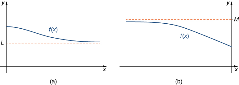
The figure is broken up into two figures labeled a and b. Figure a shows a function f(x) approaching but never touching a horizontal dashed line labeled L from above. Figure b shows a function f(x) approaching but never a horizontal dashed line labeled M from below.

Figure 2. (a) As [latex]x\to \infty[/latex], the values of [latex]f[/latex] are getting arbitrarily close to [latex]L[/latex]. The line [latex]y=L[/latex] is a horizontal asymptote of [latex]f[/latex]. (b) As [latex]x\to −\infty[/latex], the values of [latex]f[/latex] are getting arbitrarily close to [latex]M[/latex]. The line [latex]y=M[/latex] is a horizontal asymptote of [latex]f[/latex].

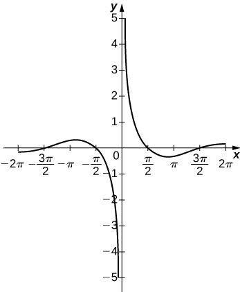
A function cannot cross a vertical asymptote because the graph must approach infinity (or negative infinity) from at least one direction as [latex]x[/latex] approaches the vertical asymptote. However, a function may cross a horizontal asymptote. In fact, a function may cross a horizontal asymptote an unlimited number of times. For example, the function [latex]f(x)=\frac{ \cos x}{x}+1[/latex] shown in (Figure) intersects the horizontal asymptote [latex]y=1[/latex] an infinite number of times as it oscillates around the asymptote with ever-decreasing amplitude.

The function f(x) = (cos x)/x + 1 is shown. It decreases from (0, ∞) and then proceeds to oscillate around y = 1 with decreasing amplitude.

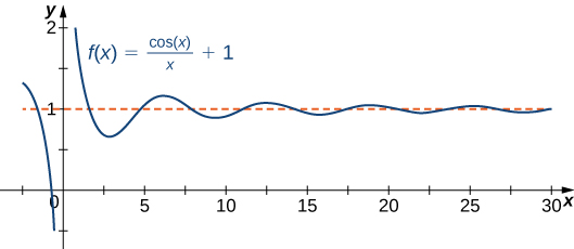
Figure 3. The graph of [latex]f(x)=\cos x/x+1[/latex] crosses its horizontal asymptote [latex]y=1[/latex] an infinite number of times.

The algebraic limit laws and squeeze theorem we introduced in Introduction to Limits also apply to limits at infinity. We illustrate how to use these laws to compute several limits at infinity.

Computing Limits at Infinity

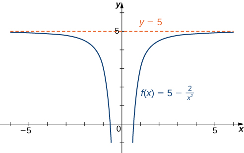
For each of the following functions [latex]f[/latex], evaluate [latex]\underset{x\to \infty }{\lim}f(x)[/latex] and [latex]\underset{x\to −\infty }{\lim}f(x)[/latex]. Determine the horizontal asymptote(s) for [latex]f[/latex].

[latex]f(x)=5-\frac{2}{x^2}[/latex]
[latex]f(x)=\frac{\sin x}{x}[/latex]
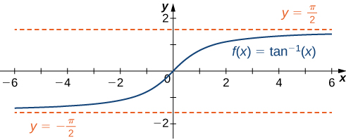
[latex]f(x)= \tan^{-1} (x)[/latex]

Show Solution

Using the algebraic limit laws, we have [latex]\underset{x\to \infty }{\lim}(5-\frac{2}{x^2})=\underset{x\to \infty }{\lim}5-2(\underset{x\to \infty }{\lim}\frac{1}{x})(\underset{x\to \infty }{\lim}\frac{1}{x})=5-2 \cdot 0=5[/latex]. Similarly, [latex]\underset{x\to \infty }{\lim}f(x)=5[/latex]. Therefore, [latex]f(x)=5-\frac{2}{x^2}[/latex] has a horizontal asymptote of [latex]y=5[/latex] and [latex]f[/latex] approaches this horizontal asymptote as [latex]x\to \pm \infty [/latex] as shown in the following graph.

Figure 4. This function approaches a horizontal asymptote as [latex]x\to \pm \infty[/latex].
Since [latex]-1\le \sin x\le 1[/latex] for all [latex]x[/latex], we have
[latex]\frac{-1}{x}\le \frac{\sin x}{x}\le \frac{1}{x}[/latex]

for all [latex]x \ne 0[/latex]. Also, since

[latex]\underset{x\to \infty }{\lim}\frac{-1}{x}=0=\underset{x\to \infty }{\lim}\frac{1}{x}[/latex],

we can apply the squeeze theorem to conclude that

[latex]\underset{x\to \infty }{\lim}\frac{\sin x}{x}=0[/latex].

Similarly,

[latex]\underset{x\to −\infty}{\lim}\frac{\sin x}{x}=0[/latex].

Thus, [latex]f(x)=\frac{\sin x}{x}[/latex] has a horizontal asymptote of [latex]y=0[/latex] and [latex]f(x)[/latex] approaches this horizontal asymptote as [latex]x\to \pm \infty [/latex] as shown in the following graph.

Figure 5. This function crosses its horizontal asymptote multiple times.
To evaluate [latex]\underset{x\to \infty }{\lim} \tan^{-1} (x)[/latex] and [latex]\underset{x\to −\infty}{\lim} \tan^{-1} (x)[/latex], we first consider the graph of [latex]y= \tan (x)[/latex] over the interval [latex](−\pi /2,\pi /2)[/latex] as shown in the following graph.

The graph of [latex] \tan x[/latex] has vertical asymptotes at [latex]x=\pm \frac{\pi }{2}[/latex]

Since

[latex]\underset{x\to (\pi/2)^-}{\lim} \tan x=\infty [/latex],

it follows that

[latex]\underset{x\to \infty }{\lim} \tan^{-1} (x)=\frac{\pi }{2}[/latex].

Similarly, since

[latex]\underset{x\to (\pi/2)^+}{\lim} \tan x=−\infty[/latex],

it follows that

[latex]\underset{x\to −\infty}{\lim} \tan^{-1} (x)=-\frac{\pi }{2}[/latex].

As a result, [latex]y=\frac{\pi }{2}[/latex] and [latex]y=-\frac{\pi }{2}[/latex] are horizontal asymptotes of [latex]f(x)= \tan^{-1} (x)[/latex] as shown in the following graph.

The function f(x) = tan−1 x is shown. It increases from (−∞, −π/2), passes through the origin, and then increases toward (∞, π/2). There are horizontal dashed lines marking y = ±π/2.

Figure 7. This function has two horizontal asymptotes.

Evaluate [latex]\underset{x\to −\infty}{\lim}(3+\frac{4}{x})[/latex] and [latex]\underset{x\to \infty }{\lim}(3+\frac{4}{x})[/latex]. Determine the horizontal asymptotes of [latex]f(x)=3+\frac{4}{x}[/latex], if any.

Show Solution

Hint

[latex]\underset{x\to \pm \infty }{\lim}1/x=0[/latex]

Infinite Limits at Infinity

Sometimes the values of a function [latex]f[/latex] become arbitrarily large as [latex]x\to \infty [/latex] (or as [latex]x\to −\infty )[/latex]. In this case, we write [latex]\underset{x\to \infty }{\lim}f(x)=\infty [/latex] (or [latex]\underset{x\to −\infty }{\lim}f(x)=\infty )[/latex]. On the other hand, if the values of [latex]f[/latex] are negative but become arbitrarily large in magnitude as [latex]x\to \infty [/latex] (or as [latex]x\to −\infty )[/latex], we write [latex]\underset{x\to \infty }{\lim}f(x)=−\infty [/latex] (or [latex]\underset{x\to −\infty }{\lim}f(x)=−\infty )[/latex].

For example, consider the function [latex]f(x)=x^3[/latex]. As seen in (Figure) and (Figure), as [latex]x\to \infty [/latex] the values [latex]f(x)[/latex] become arbitrarily large. Therefore, [latex]\underset{x\to \infty }{\lim}x^3=\infty[/latex]. On the other hand, as [latex]x\to −\infty[/latex], the values of [latex]f(x)=x^3[/latex] are negative but become arbitrarily large in magnitude. Consequently, [latex]\underset{x\to −\infty }{\lim}x^3=−\infty[/latex].

Values of a power function as [latex]x\to \pm \infty [/latex]
[latex]x[/latex]	10	20	50	100	1000
[latex]x^3[/latex]	1000	8000	125,000	1,000,000	1,000,000,000
[latex]x[/latex]	-10	-20	-50	-100	-1000
[latex]x^3[/latex]	-1000	-8000	-125,000	-1,000,000	-1,000,000,000

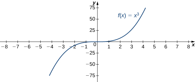
The function f(x) = x3 is graphed. It is apparent that this function rapidly approaches infinity as x approaches infinity.

Figure 8. For this function, the functional values approach infinity as [latex]x\to \pm \infty[/latex].

Definition

(Informal) We say a function [latex]f[/latex] has an infinite limit at infinity and write

[latex]\underset{x\to \infty }{\lim}f(x)=\infty [/latex].

if [latex]f(x)[/latex] becomes arbitrarily large for [latex]x[/latex] sufficiently large. We say a function has a negative infinite limit at infinity and write

[latex]\underset{x\to \infty }{\lim}f(x)=−\infty[/latex].

if [latex]f(x)<0[/latex] and [latex]|f(x)|[/latex] becomes arbitrarily large for [latex]x[/latex] sufficiently large. Similarly, we can define infinite limits as [latex]x\to −\infty[/latex].

Formal Definitions

Earlier, we used the terms arbitrarily close, arbitrarily large, and sufficiently large to define limits at infinity informally. Although these terms provide accurate descriptions of limits at infinity, they are not precise mathematically. Here are more formal definitions of limits at infinity. We then look at how to use these definitions to prove results involving limits at infinity.

Definition

(Formal) We say a function [latex]f[/latex] has a limit at infinity, if there exists a real number [latex]L[/latex] such that for all [latex]\epsilon >0[/latex], there exists [latex]N>0[/latex] such that

[latex]|f(x)-L|<\epsilon [/latex]

for all [latex]x>N[/latex]. In that case, we write

[latex]\underset{x\to \infty }{\lim}f(x)=L[/latex]

(see (Figure)).

We say a function [latex]f[/latex] has a limit at negative infinity if there exists a real number [latex]L[/latex] such that for all [latex]\epsilon >0[/latex], there exists [latex]N<0[/latex] such that

[latex]|f(x)-L|<\epsilon [/latex]

for all [latex]x<N[/latex]. In that case, we write

[latex]\underset{x\to −\infty }{\lim}f(x)=L[/latex].

The function f(x) is graphed, and it has a horizontal asymptote at L. L is marked on the y axis, as is L + ॉ and L – ॉ. On the x axis, N is marked as the value of x such that f(x) = L + ॉ.

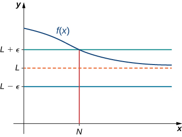
Figure 9. For a function with a limit at infinity, for all [latex]x>N[/latex], [latex]|f(x)-L|<\epsilon [/latex].

Earlier in this section, we used graphical evidence in (Figure) and numerical evidence in (Figure) to conclude that [latex]\underset{x\to \infty }{\lim}(\frac{2+1}{x})=2[/latex]. Here we use the formal definition of limit at infinity to prove this result rigorously.

A Finite Limit at Infinity Example

Use the formal definition of limit at infinity to prove that [latex]\underset{x\to \infty }{\lim}(2+\frac{1}{x})=2[/latex].

Show Solution

Use the formal definition of limit at infinity to prove that [latex]\underset{x\to \infty }{\lim}(3 - \frac{1}{x^2})=3[/latex].

Show Solution

Hint

Let [latex]N=\frac{1}{\sqrt{\epsilon }}[/latex].

We now turn our attention to a more precise definition for an infinite limit at infinity.

Definition

(Formal) We say a function [latex]f[/latex] has an infinite limit at infinity and write

[latex]\underset{x\to \infty }{\lim}f(x)=\infty [/latex]

if for all [latex]M>0[/latex], there exists an [latex]N>0[/latex] such that

[latex]f(x)>M[/latex]

for all [latex]x>N[/latex] (see (Figure)).

We say a function has a negative infinite limit at infinity and write

[latex]\underset{x\to \infty }{\lim}f(x)=−\infty [/latex]

if for all [latex]M<0[/latex], there exists an [latex]N>0[/latex] such that

[latex]f(x)<M[/latex]

for all [latex]x>N[/latex].

Similarly we can define limits as [latex]x\to −\infty[/latex].

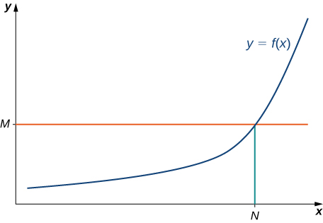
The function f(x) is graphed. It continues to increase rapidly after x = N, and f(N) = M.

Figure 10. For a function with an infinite limit at infinity, for all [latex]x>N[/latex], [latex]f(x)>M[/latex].

Earlier, we used graphical evidence ((Figure)) and numerical evidence ((Figure)) to conclude that [latex]\underset{x\to \infty }{\lim}x^3=\infty[/latex]. Here we use the formal definition of infinite limit at infinity to prove that result.

An Infinite Limit at Infinity

Use the formal definition of infinite limit at infinity to prove that [latex]\underset{x\to \infty }{\lim}x^3=\infty[/latex].

Show Solution

Use the formal definition of infinite limit at infinity to prove that [latex]\underset{x\to \infty }{\lim}3x^2=\infty[/latex].

Show Solution

Hint

Let [latex]N=\sqrt{\frac{M}{3}}[/latex].

End Behavior

The behavior of a function as [latex]x\to \pm \infty [/latex] is called the function’s end behavior. At each of the function’s ends, the function could exhibit one of the following types of behavior:

The function [latex]f(x)[/latex] approaches a horizontal asymptote [latex]y=L[/latex].
The function [latex]f(x)\to \infty [/latex] or [latex]f(x)\to −\infty[/latex].
The function does not approach a finite limit, nor does it approach [latex]\infty [/latex] or [latex]−\infty[/latex]. In this case, the function may have some oscillatory behavior.

Let’s consider several classes of functions here and look at the different types of end behaviors for these functions.

End Behavior for Polynomial Functions

Consider the power function [latex]f(x)=x^n[/latex] where [latex]n[/latex] is a positive integer. From (Figure) and (Figure), we see that

[latex]\underset{x\to \infty }{\lim}x^n=\infty; \, n=1,2,3, \cdots[/latex]

and

[latex]\underset{x\to −\infty }{\lim}x^n=\begin{cases} \infty; & n=2,4,6,\cdots \\ -\infty; & n=1,3,5,\cdots \end{cases}[/latex]

The functions x2, x4, and x6 are graphed, and it is apparent that as the exponent grows the functions increase more quickly.

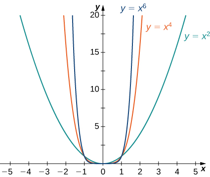
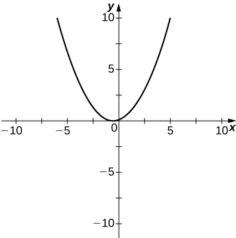
Figure 11. For power functions with an even power of [latex]n[/latex], [latex]\underset{x\to \infty }{\lim}x^n=\infty =\underset{x\to −\infty }{\lim}x^n[/latex].

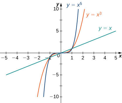
The functions x, x3, and x5 are graphed, and it is apparent that as the exponent grows the functions increase more quickly.

Figure 12. For power functions with an odd power of [latex]n[/latex], [latex]\underset{x\to \infty }{\lim}x^n=\infty [/latex] and [latex]\underset{x\to −\infty}{\lim}x^n=−\infty [/latex].

Using these facts, it is not difficult to evaluate [latex]\underset{x\to \infty }{\lim}cx^n[/latex] and [latex]\underset{x\to −\infty }{\lim}cx^n[/latex], where [latex]c[/latex] is any constant and [latex]n[/latex] is a positive integer. If [latex]c>0[/latex], the graph of [latex]y=cx^n[/latex] is a vertical stretch or compression of [latex]y=x^n[/latex], and therefore

[latex]\underset{x\to \infty }{\lim}cx^n=\underset{x\to \infty }{\lim}x^n[/latex] and [latex]\underset{x\to −\infty }{\lim}cx^n=\underset{x\to −\infty}{\lim}x^n[/latex] if [latex]c>0[/latex].

If [latex]c<0[/latex], the graph of [latex]y=cx^n[/latex] is a vertical stretch or compression combined with a reflection about the [latex]x[/latex]-axis, and therefore

[latex]\underset{x\to \infty }{\lim}cx^n=−\underset{x\to \infty }{\lim}x^n[/latex] and [latex]\underset{x\to −\infty}{\lim}cx^n=−\underset{x\to −\infty }{\lim}x^n[/latex] if [latex]c<0[/latex].

If [latex]c=0, \, y=cx^n=0[/latex], in which case [latex]\underset{x\to \infty }{\lim}cx^n=0=\underset{x\to −\infty }{\lim}cx^n[/latex].

Limits at Infinity for Power Functions

For each function [latex]f[/latex], evaluate [latex]\underset{x\to \infty }{\lim}f(x)[/latex] and [latex]\underset{x\to −\infty }{\lim}f(x)[/latex].

[latex]f(x)=-5x^3[/latex]
[latex]f(x)=2x^4[/latex]

Show Solution

Let [latex]f(x)=-3x^4[/latex]. Find [latex]\underset{x\to \infty }{\lim}f(x)[/latex].

Show Solution

Hint

The coefficient -3 is negative.

We now look at how the limits at infinity for power functions can be used to determine [latex]\underset{x\to \pm \infty }{\lim}f(x)[/latex] for any polynomial function [latex]f[/latex]. Consider a polynomial function

[latex]f(x)=a_n x^n + a_{n-1} x^{n-1} + \cdots + a_1 x + a_0[/latex]

of degree [latex]n \ge 1[/latex] so that [latex]a_n \ne 0[/latex]. Factoring, we see that

[latex]f(x)=a_n x^n (1+\frac{a_{n-1}}{a_n}\frac{1}{x}+ \cdots + \frac{a_1}{a_n}\frac{1}{x^{n-1}} + \frac{a_0}{a_n})[/latex].

As [latex]x\to \pm \infty[/latex], all the terms inside the parentheses approach zero except the first term. We conclude that

[latex]\underset{x\to \pm \infty }{\lim}f(x)=\underset{x\to \pm \infty }{\lim} a_n x^n[/latex].

For example, the function [latex]f(x)=5x^3-3x^2+4[/latex] behaves like [latex]g(x)=5x^3[/latex] as [latex]x\to \pm \infty [/latex] as shown in (Figure) and (Figure).

Both functions f(x) = 5x3 – 3x2 + 4 and g(x) = 5x3 are plotted. Their behavior for large positive and large negative numbers converges.

Figure 13. The end behavior of a polynomial is determined by the behavior of the term with the largest exponent.

A polynomial’s end behavior is determined by the term with the largest exponent.
[latex]x[/latex]	10	100	1000
[latex]f(x)=5x^3-3x^2+4[/latex]	4704	4,970,004	4,997,000,004
[latex]g(x)=5x^3[/latex]	5000	5,000,000	5,000,000,000
[latex]x[/latex]	-10	-100	-1000
[latex]f(x)=5x^3-3x^2+4[/latex]	-5296	-5,029,996	-5,002,999,996
[latex]g(x)=5x^3[/latex]	-5000	-5,000,000	-5,000,000,000

End Behavior for Algebraic Functions

The end behavior for rational functions and functions involving radicals is a little more complicated than for polynomials. In (Figure), we show that the limits at infinity of a rational function [latex]f(x)=\frac{p(x)}{q(x)}[/latex] depend on the relationship between the degree of the numerator and the degree of the denominator. To evaluate the limits at infinity for a rational function, we divide the numerator and denominator by the highest power of [latex]x[/latex] appearing in the denominator. This determines which term in the overall expression dominates the behavior of the function at large values of [latex]x[/latex].

Determining End Behavior for Rational Functions

For each of the following functions, determine the limits as [latex]x\to \infty [/latex] and [latex]x\to −\infty[/latex]. Then, use this information to describe the end behavior of the function.

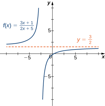
[latex]f(x)=\frac{3x-1}{2x+5}[/latex] (Note: The degree of the numerator and the denominator are the same.)
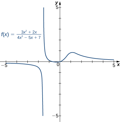
[latex]f(x)=\frac{3x^2+2x}{4x^3-5x+7}[/latex] (Note: The degree of numerator is less than the degree of the denominator.)
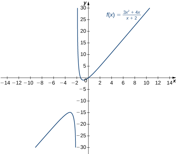
[latex]f(x)=\frac{3x^2+4x}{x+2}[/latex] (Note: The degree of numerator is greater than the degree of the denominator.)

Show Solution

The highest power of [latex]x[/latex] in the denominator is [latex]x[/latex]. Therefore, dividing the numerator and denominator by [latex]x[/latex] and applying the algebraic limit laws, we see that
[latex]\begin{array}{ll} \underset{x\to \pm \infty }{\lim}\frac{3x-1}{2x+5} & =\underset{x\to \pm \infty }{\lim}\frac{3-1/x}{2+5/x} \\ & =\frac{\underset{x\to \pm \infty }{\lim}(3-1/x)}{\underset{x\to \pm \infty }{\lim}(2+5/x)} \\ & =\frac{\underset{x\to \pm \infty }{\lim}3-\underset{x\to \pm \infty }{\lim}1/x}{\underset{x\to \pm \infty }{\lim}2+\underset{x\to \pm \infty }{\lim}5/x} \\ & =\frac{3-0}{2+0}=\frac{3}{2}. \end{array}[/latex]

Since [latex]\underset{x\to \pm \infty }{\lim}f(x)=\frac{3}{2}[/latex], we know that [latex]y=\frac{3}{2}[/latex] is a horizontal asymptote for this function as shown in the following graph.

Figure 14. The graph of this rational function approaches a horizontal asymptote as [latex]x\to \pm \infty[/latex].
Since the largest power of [latex]x[/latex] appearing in the denominator is [latex]x^3[/latex], divide the numerator and denominator by [latex]x^3[/latex]. After doing so and applying algebraic limit laws, we obtain
[latex]\underset{x\to \pm \infty }{\lim}\frac{3x^2+2x}{4x^3-5x+7}=\underset{x\to \pm \infty }{\lim}\frac{3/x+2/x^2}{4-5/x^2+7/x^3}=\frac{3 \cdot 0+2 \cdot 0}{4-5 \cdot 0+7 c\dot 0}=0[/latex]

Therefore [latex]f[/latex] has a horizontal asymptote of [latex]y=0[/latex] as shown in the following graph.

Figure 15. The graph of this rational function approaches the horizontal asymptote [latex]y=0[/latex] as [latex]x\to \pm \infty[/latex].
Dividing the numerator and denominator by [latex]x[/latex], we have
[latex]\underset{x\to \pm \infty }{\lim}\frac{3x^2+4x}{x+2}=\underset{x\to \pm \infty }{\lim}\frac{3x+4}{1+2/x}[/latex].

As [latex]x\to \pm \infty[/latex], the denominator approaches 1. As [latex]x\to \infty[/latex], the numerator approaches [latex]+\infty[/latex]. As [latex]x\to −\infty[/latex], the numerator approaches [latex]−\infty[/latex]. Therefore [latex]\underset{x\to \infty }{\lim}f(x)=\infty[/latex], whereas [latex]\underset{x\to −\infty }{\lim}f(x)=−\infty [/latex] as shown in the following figure.

Figure 16. As [latex]x\to \infty[/latex], the values [latex]f(x)\to \infty[/latex]. As [latex]x\to −\infty[/latex], the values [latex]f(x)\to −\infty[/latex].

Evaluate [latex]\underset{x\to \pm \infty }{\lim}\frac{3x^2+2x-1}{5x^2-4x+7}[/latex] and use these limits to determine the end behavior of [latex]f(x)=\frac{3x^2+2x-2}{5x^2-4x+7}[/latex].

Show Solution

Hint

Divide the numerator and denominator by [latex]x^2[/latex].

Before proceeding, consider the graph of [latex]f(x)=\frac{(3x^2+4x)}{(x+2)}[/latex] shown in (Figure). As [latex]x\to \infty [/latex] and [latex]x\to −\infty[/latex], the graph of [latex]f[/latex] appears almost linear. Although [latex]f[/latex] is certainly not a linear function, we now investigate why the graph of [latex]f[/latex] seems to be approaching a linear function. First, using long division of polynomials, we can write

[latex]f(x)=\frac{3x^2+4x}{x+2}=3x-2+\frac{4}{x+2}[/latex].

Since [latex]\frac{4}{(x+2)}\to 0[/latex] as [latex]x\to \pm \infty[/latex], we conclude that

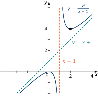
[latex]\underset{x\to \pm \infty }{\lim}(f(x)-(3x-2))=\underset{x\to \pm \infty }{\lim}\frac{4}{x+2}=0[/latex].

Therefore, the graph of [latex]f[/latex] approaches the line [latex]y=3x-2[/latex] as [latex]x\to \pm \infty[/latex]. This line is known as an oblique asymptote for [latex]f[/latex] ((Figure)).

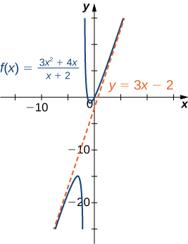
The function f(x) = (3x2 + 4x)/(x + 2) is plotted as is its diagonal asymptote y = 3x – 2.

Figure 17. The graph of the rational function [latex]f(x)=(3x^2+4x)/(x+2)[/latex] approaches the oblique asymptote [latex]y=3x-2[/latex] as [latex]x\to \pm \infty[/latex].

We can summarize the results of (Figure) to make the following conclusion regarding end behavior for rational functions. Consider a rational function

[latex]f(x)=\frac{p(x)}{q(x)}=\frac{a_n x^n + a_{n-1} x^{n-1} + \cdots + a_1 x + a_0}{b_m x^m + b_{m-1} x^{m-1} + \cdots + b_1 x + b_0}[/latex],

where [latex]a_n\ne 0[/latex] and [latex]b_m \ne 0[/latex].

If the degree of the numerator is the same as the degree of the denominator [latex](n=m)[/latex], then [latex]f[/latex] has a horizontal asymptote of [latex]y=a_n/b_m[/latex] as [latex]x\to \pm \infty[/latex].
If the degree of the numerator is less than the degree of the denominator [latex](n<m)[/latex], then [latex]f[/latex] has a horizontal asymptote of [latex]y=0[/latex] as [latex]x\to \pm \infty[/latex].
If the degree of the numerator is greater than the degree of the denominator [latex](n>m)[/latex], then [latex]f[/latex] does not have a horizontal asymptote. The limits at infinity are either positive or negative infinity, depending on the signs of the leading terms. In addition, using long division, the function can be rewritten as
[latex]f(x)=\frac{p(x)}{q(x)}=g(x)+\frac{r(x)}{q(x)}[/latex],

where the degree of [latex]r(x)[/latex] is less than the degree of [latex]q(x)[/latex]. As a result, [latex]\underset{x\to \pm \infty }{\lim}r(x)/q(x)=0[/latex]. Therefore, the values of [latex][f(x)-g(x)][/latex] approach zero as [latex]x\to \pm \infty[/latex]. If the degree of [latex]p(x)[/latex] is exactly one more than the degree of [latex]q(x)[/latex] [latex](n=m+1)[/latex], the function [latex]g(x)[/latex] is a linear function. In this case, we call [latex]g(x)[/latex] an oblique asymptote.
Now let’s consider the end behavior for functions involving a radical.

Determining End Behavior for a Function Involving a Radical

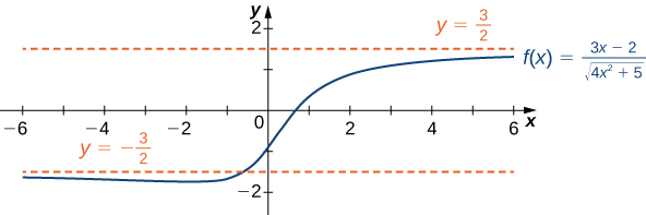
Find the limits as [latex]x\to \infty [/latex] and [latex]x\to −\infty [/latex] for [latex]f(x)=\frac{3x-2}{\sqrt{4x^2+5}}[/latex] and describe the end behavior of [latex]f[/latex].

Show Solution

Evaluate [latex]\underset{x\to \infty }{\lim}\frac{\sqrt{3x^2+4}}{x+6}[/latex].

Show Solution

Hint

Divide the numerator and denominator by [latex]|x|[/latex].

Determining End Behavior for Transcendental Functions

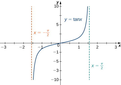
The six basic trigonometric functions are periodic and do not approach a finite limit as [latex]x\to \pm \infty[/latex]. For example, [latex]\sin x[/latex] oscillates between 1 and -1 ((Figure)). The tangent function [latex]x[/latex] has an infinite number of vertical asymptotes as [latex]x\to \pm \infty[/latex]; therefore, it does not approach a finite limit nor does it approach [latex]\pm \infty [/latex] as [latex]x\to \pm \infty [/latex] as shown in (Figure).

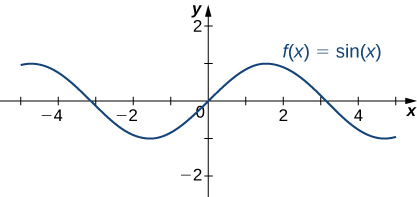
Figure 19. The function [latex]f(x)= \sin x[/latex] oscillates between 1 and -1 as [latex]x\to \pm \infty [/latex]

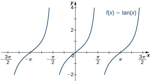
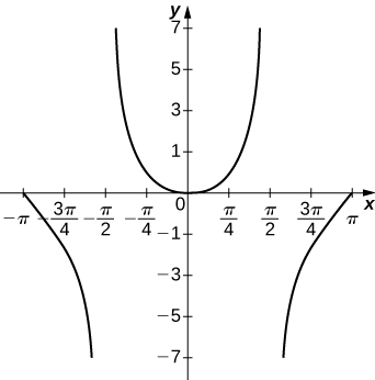
Figure 20. The function [latex]f(x)= \tan x[/latex] does not approach a limit and does not approach [latex]\pm \infty [/latex] as [latex]x\to \pm \infty [/latex]

Recall that for any base [latex]b>0, \, b\ne 1[/latex], the function [latex]y=b^x[/latex] is an exponential function with domain [latex](−\infty ,\infty )[/latex] and range [latex](0,\infty )[/latex]. If [latex]b>1, \, y=b^x[/latex] is increasing over [latex](−\infty ,\infty )[/latex]. If [latex]0<b<1[/latex], [latex]y=b^x[/latex] is decreasing over [latex](−\infty ,\infty )[/latex]. For the natural exponential function [latex]f(x)=e^x[/latex], [latex]e\approx 2.718>1[/latex]. Therefore, [latex]f(x)=e^x[/latex] is increasing on [latex](−\infty ,\infty )[/latex] and the range is [latex](0,\infty)[/latex]. The exponential function [latex]f(x)=e^x[/latex] approaches [latex]\infty [/latex] as [latex]x\to \infty [/latex] and approaches 0 as [latex]x\to −\infty [/latex] as shown in (Figure) and (Figure).

End behavior of the natural exponential function
[latex]x[/latex]	-5	-2	0	2	5
[latex]e^x[/latex]	0.00674	0.135	1	7.389	148.413

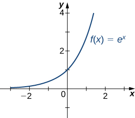
Figure 21. The exponential function approaches zero as [latex]x\to −\infty [/latex] and approaches [latex]\infty [/latex] as [latex]x\to \infty[/latex].

Recall that the natural logarithm function [latex]f(x)=\ln (x)[/latex] is the inverse of the natural exponential function [latex]y=e^x[/latex]. Therefore, the domain of [latex]f(x)=\ln (x)[/latex] is [latex](0,\infty )[/latex] and the range is [latex](−\infty ,\infty )[/latex]. The graph of [latex]f(x)=\ln (x)[/latex] is the reflection of the graph of [latex]y=e^x[/latex] about the line [latex]y=x[/latex]. Therefore, [latex]\ln (x)\to −\infty [/latex] as [latex]x\to 0^+[/latex] and [latex]\ln (x)\to \infty [/latex] as [latex]x\to \infty [/latex] as shown in (Figure) and (Figure).

End behavior of the natural logarithm function
[latex]x[/latex]	0.01	0.1	1	10	100
[latex]\ln (x)[/latex]	-4.605	-2.303	0	2.303	4.605

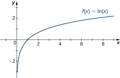
Figure 22. The natural logarithm function approaches [latex]\infty [/latex] as [latex]x\to \infty[/latex].

Determining End Behavior for a Transcendental Function

Find the limits as [latex]x\to \infty [/latex] and [latex]x\to −\infty [/latex] for [latex]f(x)=\frac{(2+3e^x)}{(7-5e^x)}[/latex] and describe the end behavior of [latex]f[/latex].

Show Solution

Find the limits as [latex]x\to \infty [/latex] and [latex]x\to −\infty [/latex] for [latex]f(x)=\frac{(3e^x-4)}{(5e^x+2)}[/latex].

Show Solution

Hint

[latex]\underset{x\to \infty }{\lim}e^x=\infty [/latex] and [latex]\underset{x\to -\infty }{\lim}e^x=0[/latex].

Guidelines for Drawing the Graph of a Function

We now have enough analytical tools to draw graphs of a wide variety of algebraic and transcendental functions. Before showing how to graph specific functions, let’s look at a general strategy to use when graphing any function.

Problem-Solving Strategy: Drawing the Graph of a Function

Given a function [latex]f[/latex] use the following steps to sketch a graph of [latex]f[/latex]:

Determine the domain of the function.
Locate the [latex]x[/latex]– and [latex]y[/latex]-intercepts.
Evaluate [latex]\underset{x\to \infty }{\lim}f(x)[/latex] and [latex]\underset{x\to −\infty }{\lim}f(x)[/latex] to determine the end behavior. If either of these limits is a finite number [latex]L[/latex], then [latex]y=L[/latex] is a horizontal asymptote. If either of these limits is [latex]\infty [/latex] or [latex]−\infty[/latex], determine whether [latex]f[/latex] has an oblique asymptote. If [latex]f[/latex] is a rational function such that [latex]f(x)=\frac{p(x)}{q(x)}[/latex], where the degree of the numerator is greater than the degree of the denominator, then [latex]f[/latex] can be written as
[latex]f(x)=\frac{p(x)}{q(x)}=g(x)+\frac{r(x)}{q(x)}[/latex],

where the degree of [latex]r(x)[/latex] is less than the degree of [latex]q(x)[/latex]. The values of [latex]f(x)[/latex] approach the values of [latex]g(x)[/latex] as [latex]x\to \pm \infty[/latex]. If [latex]g(x)[/latex] is a linear function, it is known as an oblique asymptote.
Determine whether [latex]f[/latex] has any vertical asymptotes.
Calculate [latex]f^{\prime}[/latex]. Find all critical points and determine the intervals where [latex]f[/latex] is increasing and where [latex]f[/latex] is decreasing. Determine whether [latex]f[/latex] has any local extrema.
Calculate [latex]f^{\prime \prime}[/latex]. Determine the intervals where [latex]f[/latex] is concave up and where [latex]f[/latex] is concave down. Use this information to determine whether [latex]f[/latex] has any inflection points. The second derivative can also be used as an alternate means to determine or verify that [latex]f[/latex] has a local extremum at a critical point.

Now let’s use this strategy to graph several different functions. We start by graphing a polynomial function.

Sketching a Graph of a Polynomial

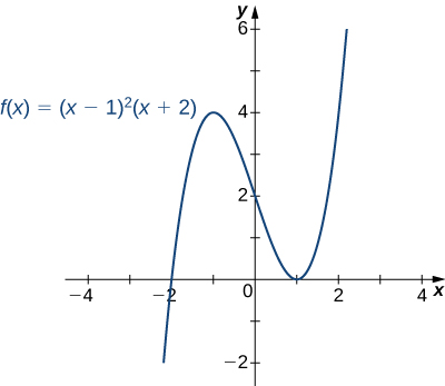
Sketch a graph of [latex]f(x)=(x-1)^2 (x+2)[/latex].

Show Solution

Step 1. Since [latex]f[/latex] is a polynomial, the domain is the set of all real numbers.

Step 2. When [latex]x=0, \, f(x)=2[/latex]. Therefore, the [latex]y[/latex]-intercept is [latex](0,2)[/latex]. To find the [latex]x[/latex]-intercepts, we need to solve the equation [latex](x-1)^2 (x+2)=0[/latex], which gives us the [latex]x[/latex]-intercepts [latex](1,0)[/latex] and [latex](-2,0)[/latex]

Step 3. We need to evaluate the end behavior of [latex]f[/latex]. As [latex]x\to \infty[/latex], [latex](x-1)^2 \to \infty [/latex] and [latex](x+2)\to \infty[/latex]. Therefore, [latex]\underset{x\to \infty }{\lim}f(x)=\infty[/latex]. As [latex]x\to −\infty[/latex], [latex](x-1)^2 \to \infty [/latex] and [latex](x+2) \to −\infty[/latex]. Therefore, [latex]\underset{x\to -\infty }{\lim}f(x)=−\infty[/latex]. To get even more information about the end behavior of [latex]f[/latex], we can multiply the factors of [latex]f[/latex]. When doing so, we see that

[latex]f(x)=(x-1)^2 (x+2)=x^3-3x+2[/latex].

Since the leading term of [latex]f[/latex] is [latex]x^3[/latex], we conclude that [latex]f[/latex] behaves like [latex]y=x^3[/latex] as [latex]x\to \pm \infty[/latex].

Step 4. Since [latex]f[/latex] is a polynomial function, it does not have any vertical asymptotes.

Step 5. The first derivative of [latex]f[/latex] is

[latex]f^{\prime}(x)=3x^2-3[/latex].

Therefore, [latex]f[/latex] has two critical points: [latex]x=1,-1[/latex]. Divide the interval [latex](−\infty ,\infty)[/latex] into the three smaller intervals: [latex](−\infty ,-1)[/latex], [latex](-1,1)[/latex], and [latex](1,\infty )[/latex]. Then, choose test points [latex]x=-2[/latex], [latex]x=0[/latex], and [latex]x=2[/latex] from these intervals and evaluate the sign of [latex]f^{\prime}(x)[/latex] at each of these test points, as shown in the following table.

Interval	Test Point	Sign of Derivative [latex]f^{\prime}(x)=3x^2-3=3(x-1)(x+1)[/latex]	Conclusion
[latex](−\infty ,-1)[/latex]	[latex]x=-2[/latex]	[latex](+)(−)(−)=+[/latex]	[latex]f[/latex] is increasing.
[latex](-1,1)[/latex]	[latex]x=0[/latex]	[latex](+)(−)(+)=−[/latex]	[latex]f[/latex] is decreasing.
[latex](1,\infty )[/latex]	[latex]x=2[/latex]	[latex](+)(+)(+)=+[/latex]	[latex]f[/latex] is increasing.

From the table, we see that [latex]f[/latex] has a local maximum at [latex]x=-1[/latex] and a local minimum at [latex]x=1[/latex]. Evaluating [latex]f(x)[/latex] at those two points, we find that the local maximum value is [latex]f(-1)=4[/latex] and the local minimum value is [latex]f(1)=0[/latex].

Step 6. The second derivative of [latex]f[/latex] is

[latex]f^{\prime \prime}(x)=6x[/latex].

The second derivative is zero at [latex]x=0[/latex]. Therefore, to determine the concavity of [latex]f[/latex], divide the interval [latex](−\infty ,\infty)[/latex] into the smaller intervals [latex](−\infty ,0)[/latex] and [latex](0,\infty )[/latex], and choose test points [latex]x=-1[/latex] and [latex]x=1[/latex] to determine the concavity of [latex]f[/latex] on each of these smaller intervals as shown in the following table.

Interval	Test Point	Sign of [latex]f^{\prime \prime}(x)=6x[/latex]	Conclusion
[latex](−\infty ,0)[/latex]	[latex]x=-1[/latex]	[latex]-[/latex]	[latex]f[/latex] is concave down.
[latex](0,\infty )[/latex]	[latex]x=1[/latex]	[latex]+[/latex]	[latex]f[/latex] is concave up.

We note that the information in the preceding table confirms the fact, found in step 5, that [latex]f[/latex] has a local maximum at [latex]x=-1[/latex] and a local minimum at [latex]x=1[/latex]. In addition, the information found in step 5—namely, [latex]f[/latex] has a local maximum at [latex]x=-1[/latex] and a local minimum at [latex]x=1[/latex], and [latex]f^{\prime}(x)=0[/latex] at those points—combined with the fact that [latex]f^{\prime \prime}[/latex] changes sign only at [latex]x=0[/latex] confirms the results found in step 6 on the concavity of [latex]f[/latex].

Combining this information, we arrive at the graph of [latex]f(x)=(x-1)^2 (x+2)[/latex] shown in the following graph.

The function f(x) = (x −1)2 (x + 2) is graphed. It crosses the x axis at x = −2 and touches the x axis at x = 1.

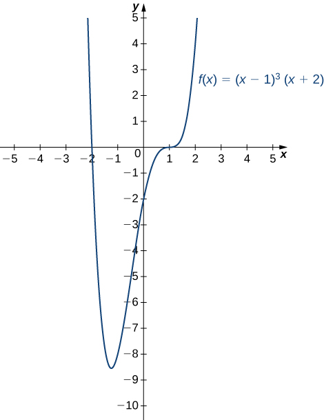
Sketch a graph of [latex]f(x)=(x-1)^3 (x+2)[/latex].

Show Solution

Hint

[latex]f[/latex] is a fourth-degree polynomial.

Sketching a Rational Function

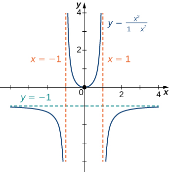
Sketch the graph of [latex]f(x)=\frac{x^2}{1-x^2}[/latex].

Show Solution

Step 1. The function [latex]f[/latex] is defined as long as the denominator is not zero. Therefore, the domain is the set of all real numbers [latex]x[/latex] except [latex]x=\pm 1[/latex].

Step 2. Find the intercepts. If [latex]x=0[/latex], then [latex]f(x)=0[/latex], so 0 is an intercept. If [latex]y=0[/latex], then [latex]\frac{x^2}{1-x^2}=0[/latex], which implies [latex]x=0[/latex]. Therefore, [latex](0,0)[/latex] is the only intercept.

Step 3. Evaluate the limits at infinity. Since [latex]f[/latex] is a rational function, divide the numerator and denominator by the highest power in the denominator: [latex]x^2[/latex]. We obtain

[latex]\underset{x\to \pm \infty }{\lim}\frac{x^2}{1-x^2}=\underset{x\to \pm \infty }{\lim}\frac{1}{\frac{1}{x^2}-1}=-1[/latex].

Therefore, [latex]f[/latex] has a horizontal asymptote of [latex]y=-1[/latex] as [latex]x\to \infty [/latex] and [latex]x\to −\infty[/latex].

Step 4. To determine whether [latex]f[/latex] has any vertical asymptotes, first check to see whether the denominator has any zeroes. We find the denominator is zero when [latex]x=\pm 1[/latex]. To determine whether the lines [latex]x=1[/latex] or [latex]x=-1[/latex] are vertical asymptotes of [latex]f[/latex], evaluate [latex]\underset{x\to 1}{\lim}f(x)[/latex] and [latex]\underset{x\to −1}{\lim}f(x)[/latex]. By looking at each one-sided limit as [latex]x\to 1[/latex], we see that

[latex]\underset{x\to 1^+}{\lim}\frac{x^2}{1-x^2}=−\infty[/latex] and [latex]\underset{x\to 1^-}{\lim}\frac{x^2}{1-x^2}=\infty[/latex].

In addition, by looking at each one-sided limit as [latex]x\to −1[/latex], we find that

[latex]\underset{x\to −1^+}{\lim}\frac{x^2}{1-x^2}=\infty[/latex] and [latex]\underset{x\to −1^-}{\lim}\frac{x^2}{1-x^2}=−\infty[/latex].

Step 5. Calculate the first derivative:

[latex]f^{\prime}(x)=\frac{(1-x^2)(2x)-x^2(-2x)}{(1-x^2)^2}=\frac{2x}{(1-x^2)^2}[/latex].

Critical points occur at points [latex]x[/latex] where [latex]f^{\prime}(x)=0[/latex] or [latex]f^{\prime}(x)[/latex] is undefined. We see that [latex]f^{\prime}(x)=0[/latex] when [latex]x=0[/latex]. The derivative [latex]f^{\prime}[/latex] is not undefined at any point in the domain of [latex]f[/latex]. However, [latex]x=\pm 1[/latex] are not in the domain of [latex]f[/latex]. Therefore, to determine where [latex]f[/latex] is increasing and where [latex]f[/latex] is decreasing, divide the interval [latex](−\infty ,\infty )[/latex] into four smaller intervals: [latex](−\infty ,-1)[/latex], [latex](-1,0)[/latex], [latex](0,1)[/latex], and [latex](1,\infty )[/latex], and choose a test point in each interval to determine the sign of [latex]f^{\prime}(x)[/latex] in each of these intervals. The values [latex]x=-2[/latex], [latex]x=-\frac{1}{2}[/latex], [latex]x=\frac{1}{2}[/latex], and [latex]x=2[/latex] are good choices for test points as shown in the following table.

Interval	Test Point	Sign of [latex]f^{\prime}(x)=\frac{2x}{(1-x^2)^2}[/latex]	Conclusion
[latex](−\infty ,-1)[/latex]	[latex]x=-2[/latex]	[latex]−/+=−[/latex]	[latex]f[/latex] is decreasing.
[latex](-1,0)[/latex]	[latex]x=-1/2[/latex]	[latex]−/+=−[/latex]	[latex]f[/latex] is decreasing.
[latex](0,1)[/latex]	[latex]x=1/2[/latex]	[latex]+/+=+[/latex]	[latex]f[/latex] is increasing.
[latex](1,\infty )[/latex]	[latex]x=2[/latex]	[latex]+/+=+[/latex]	[latex]f[/latex] is increasing.

From this analysis, we conclude that [latex]f[/latex] has a local minimum at [latex]x=0[/latex] but no local maximum.

Step 6. Calculate the second derivative:

[latex]\begin{array}{ll} f^{\prime \prime}(x) & =\frac{(1-x^2)^2(2)-2x(2(1-x^2)(-2x))}{(1-x^2)^4} \\ & =\frac{(1-x^2)[2(1-x^2)+8x^2]}{(1-x^2)^4} \\ & =\frac{2(1-x^2)+8x^2}{(1-x^2)^3} \\ & =\frac{6x^2+2}{(1-x^2)^3} \end{array}[/latex]

To determine the intervals where [latex]f[/latex] is concave up and where [latex]f[/latex] is concave down, we first need to find all points [latex]x[/latex] where [latex]f^{\prime \prime}(x)=0[/latex] or [latex]f^{\prime \prime}(x)[/latex] is undefined. Since the numerator [latex]6x^2+2 \ne 0[/latex] for any [latex]x[/latex], [latex]f^{\prime \prime}(x)[/latex] is never zero. Furthermore, [latex]f^{\prime \prime}[/latex] is not undefined for any [latex]x[/latex] in the domain of [latex]f[/latex]. However, as discussed earlier, [latex]x=\pm 1[/latex] are not in the domain of [latex]f[/latex]. Therefore, to determine the concavity of [latex]f[/latex], we divide the interval [latex](−\infty ,\infty )[/latex] into the three smaller intervals [latex](−\infty ,-1)[/latex], [latex](-1,-1)[/latex], and [latex](1,\infty )[/latex], and choose a test point in each of these intervals to evaluate the sign of [latex]f^{\prime \prime}(x)[/latex] in each of these intervals. The values [latex]x=-2[/latex], [latex]x=0[/latex], and [latex]x=2[/latex] are possible test points as shown in the following table.

Interval	Test Point	Sign of [latex]f^{\prime \prime}(x)=\frac{6x^2+2}{(1-x^2)^3}[/latex]	Conclusion
[latex](−\infty ,-1)[/latex]	[latex]x=-2[/latex]	[latex]+/-=−[/latex]	[latex]f[/latex] is concave down.
[latex](-1,-1)[/latex]	[latex]x=0[/latex]	[latex]+/+=+[/latex]	[latex]f[/latex] is concave up.
[latex](1,\infty )[/latex]	[latex]x=2[/latex]	[latex]+/-=−[/latex]	[latex]f[/latex] is concave down.

Combining all this information, we arrive at the graph of [latex]f[/latex] shown below. Note that, although [latex]f[/latex] changes concavity at [latex]x=-1[/latex] and [latex]x=1[/latex], there are no inflection points at either of these places because [latex]f[/latex] is not continuous at [latex]x=-1[/latex] or [latex]x=1[/latex].

The function f(x) = x2/(1 − x2) is graphed. It has asymptotes y = −1, x = −1, and x = 1.

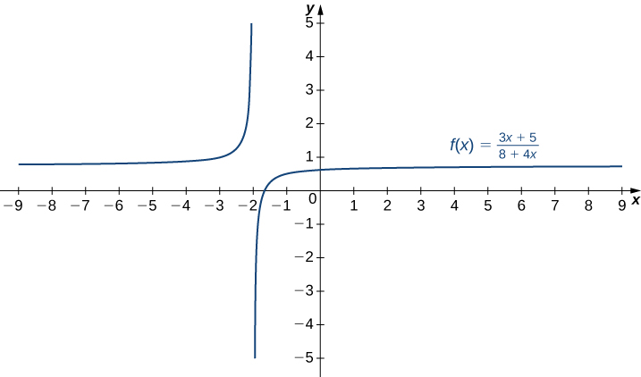
Sketch a graph of [latex]f(x)=\frac{3x+5}{8+4x}[/latex].

Show Solution

Hint

A line [latex]y=L[/latex] is a horizontal asymptote of [latex]f[/latex] if the limit as [latex]x\to \infty [/latex] or the limit as [latex]x\to −\infty [/latex] of [latex]f(x)[/latex] is [latex]L[/latex]. A line [latex]x=a[/latex] is a vertical asymptote if at least one of the one-sided limits of [latex]f[/latex] as [latex]x\to a[/latex] is [latex]\infty [/latex] or [latex]−\infty[/latex].

Sketching a Rational Function with an Oblique Asymptote

Sketch the graph of [latex]f(x)=\frac{x^2}{x-1}[/latex]

Show Solution

Step 1. The domain of [latex]f[/latex] is the set of all real numbers [latex]x[/latex] except [latex]x=1[/latex].

Step 2. Find the intercepts. We can see that when [latex]x=0[/latex], [latex]f(x)=0[/latex], so [latex](0,0)[/latex] is the only intercept.

Step 3. Evaluate the limits at infinity. Since the degree of the numerator is one more than the degree of the denominator, [latex]f[/latex] must have an oblique asymptote. To find the oblique asymptote, use long division of polynomials to write

[latex]f(x)=\frac{x^2}{x-1}=x+1+\frac{1}{x-1}[/latex].

Since [latex]1/(x-1)\to 0[/latex] as [latex]x\to \pm \infty[/latex], [latex]f(x)[/latex] approaches the line [latex]y=x+1[/latex] as [latex]x\to \pm \infty[/latex]. The line [latex]y=x+1[/latex] is an oblique asymptote for [latex]f[/latex].

Step 4. To check for vertical asymptotes, look at where the denominator is zero. Here the denominator is zero at [latex]x=1[/latex]. Looking at both one-sided limits as [latex]x\to 1[/latex], we find

[latex]\underset{x\to 1^+}{\lim}\frac{x^2}{x-1}=\infty[/latex] and [latex]\underset{x\to 1^-}{\lim}\frac{x^2}{x-1}=−\infty[/latex].

Therefore, [latex]x=1[/latex] is a vertical asymptote, and we have determined the behavior of [latex]f[/latex] as [latex]x[/latex] approaches 1 from the right and the left.

Step 5. Calculate the first derivative:

[latex]f^{\prime}(x)=\frac{(x-1)(2x)-x^2(1)}{(x-1)^2}=\frac{x^2-2x}{(x-1)^2}[/latex].

We have [latex]f^{\prime}(x)=0[/latex] when [latex]x^2-2x=x(x-2)=0[/latex]. Therefore, [latex]x=0[/latex] and [latex]x=2[/latex] are critical points. Since [latex]f[/latex] is undefined at [latex]x=1[/latex], we need to divide the interval [latex](−\infty ,\infty )[/latex] into the smaller intervals [latex](−\infty ,0)[/latex], [latex](0,1)[/latex], [latex](1,2)[/latex], and [latex](2,\infty )[/latex], and choose a test point from each interval to evaluate the sign of [latex]f^{\prime}(x)[/latex] in each of these smaller intervals. For example, let [latex]x=-1[/latex], [latex]x=\frac{1}{2}[/latex], [latex]x=\frac{3}{2}[/latex], and [latex]x=3[/latex] be the test points as shown in the following table.

Interval	Test Point	Sign of [latex]f^{\prime}(x)=\frac{x^2-2x}{(x-1)^2}=\frac{x(x-2)}{(x-1)^2}[/latex]	Conclusion
[latex](−\infty ,0)[/latex]	[latex]x=-1[/latex]	[latex](−)(−)/+=+[/latex]	[latex]f[/latex] is increasing.
[latex](0,1)[/latex]	[latex]x=1/2[/latex]	[latex](+)(−)/+=−[/latex]	[latex]f[/latex] is decreasing.
[latex](1,2)[/latex]	[latex]x=3/2[/latex]	[latex](+)(−)/+=−[/latex]	[latex]f[/latex] is decreasing.
[latex](2,\infty )[/latex]	[latex]x=3[/latex]	[latex](+)(+)/+=+[/latex]	[latex]f[/latex] is increasing.

From this table, we see that [latex]f[/latex] has a local maximum at [latex]x=0[/latex] and a local minimum at [latex]x=2[/latex]. The value of [latex]f[/latex] at the local maximum is [latex]f(0)=0[/latex] and the value of [latex]f[/latex] at the local minimum is [latex]f(2)=4[/latex]. Therefore, [latex](0,0)[/latex] and [latex](2,4)[/latex] are important points on the graph.

Step 6. Calculate the second derivative:

[latex]\begin{array}{ll} f^{\prime \prime}(x) & =\frac{(x-1)^2(2x-2)-(x^2-2x)(2(x-1))}{(x-1)^4} \\ & =\frac{(x-1)[(x-1)(2x-2)-2(x^2-2x)]}{(x-1)^4} \\ & =\frac{(x-1)(2x-2)-2(x^2-2x)}{(x-1)^3} \\ & =\frac{2x^2-4x+2-(2x^2-4x)}{(x-1)^3} \\ & =\frac{2}{(x-1)^3} \end{array}[/latex]

We see that [latex]f^{\prime \prime}(x)[/latex] is never zero or undefined for [latex]x[/latex] in the domain of [latex]f[/latex]. Since [latex]f[/latex] is undefined at [latex]x=1[/latex], to check concavity we just divide the interval [latex](−\infty ,\infty )[/latex] into the two smaller intervals [latex](−\infty ,1)[/latex] and [latex](1,\infty )[/latex], and choose a test point from each interval to evaluate the sign of [latex]f^{\prime \prime}(x)[/latex] in each of these intervals. The values [latex]x=0[/latex] and [latex]x=2[/latex] are possible test points as shown in the following table.

Interval	Test Point	Sign of [latex]f^{\prime \prime}(x)=\frac{2}{(x-1)^3}[/latex]	Conclusion
[latex](−\infty ,1)[/latex]	[latex]x=0[/latex]	[latex]+/-=−[/latex]	[latex]f[/latex] is concave down.
[latex](1,\infty )[/latex]	[latex]x=2[/latex]	[latex]+/+=+[/latex]	[latex]f[/latex] is concave up.

From the information gathered, we arrive at the following graph for [latex]f.[/latex]

The function f(x) = x2/(x − 1) is graphed. It has asymptotes y = x + 1 and x = 1.

Find the oblique asymptote for [latex]f(x)=\frac{3x^3-2x+1}{2x^2-4}[/latex].

Show Solution

Hint

Use long division of polynomials.

Sketching the Graph of a Function with a Cusp

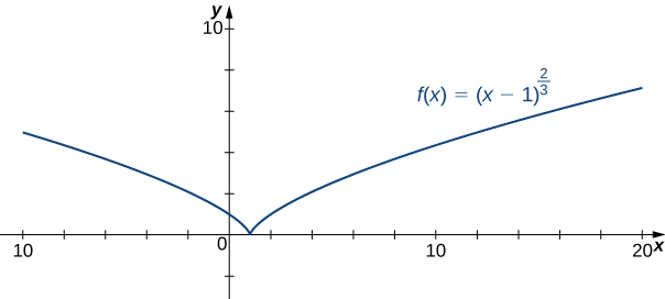
Sketch a graph of [latex]f(x)=(x-1)^{2/3}[/latex].

Show Solution

Step 1. Since the cube-root function is defined for all real numbers [latex]x[/latex] and [latex](x-1)^{2/3}=(\sqrt[3]{x-1})^2[/latex], the domain of [latex]f[/latex] is all real numbers.

Step 2: To find the [latex]y[/latex]-intercept, evaluate [latex]f(0)[/latex]. Since [latex]f(0)=1[/latex], the [latex]y[/latex]-intercept is [latex](0,1)[/latex]. To find the [latex]x[/latex]-intercept, solve [latex](x-1)^{2/3}=0[/latex]. The solution of this equation is [latex]x=1[/latex], so the [latex]x[/latex]-intercept is [latex](1,0)[/latex].

Step 3: Since [latex]\underset{x\to \pm \infty }{\lim}(x-1)^{2/3}=\infty [/latex], the function continues to grow without bound as [latex]x\to \infty [/latex] and [latex]x\to −\infty[/latex].

Step 4: The function has no vertical asymptotes.

Step 5: To determine where [latex]f[/latex] is increasing or decreasing, calculate [latex]f^{\prime}[/latex]. We find

[latex]f^{\prime}(x)=\frac{2}{3}(x-1)^{-1/3}=\frac{2}{3(x-1)^{1/3}}[/latex].

This function is not zero anywhere, but it is undefined when [latex]x=1[/latex]. Therefore, the only critical point is [latex]x=1[/latex]. Divide the interval [latex](−\infty ,\infty )[/latex] into the smaller intervals [latex](−\infty ,1)[/latex] and [latex](1,\infty )[/latex], and choose test points in each of these intervals to determine the sign of [latex]f^{\prime}(x)[/latex] in each of these smaller intervals. Let [latex]x=0[/latex] and [latex]x=2[/latex] be the test points as shown in the following table.

Interval	Test Point	Sign of [latex]f^{\prime}(x)=\frac{2}{3(x-1)^{1/3}}[/latex]	Conclusion
[latex](−\infty ,1)[/latex]	[latex]x=0[/latex]	[latex]+/-=−[/latex]	[latex]f[/latex] is decreasing.
[latex](1,\infty )[/latex]	[latex]x=2[/latex]	[latex]+/+=+[/latex]	[latex]f[/latex] is increasing.

We conclude that [latex]f[/latex] has a local minimum at [latex]x=1[/latex]. Evaluating [latex]f[/latex] at [latex]x=1[/latex], we find that the value of [latex]f[/latex] at the local minimum is zero. Note that [latex]f^{\prime}(1)[/latex] is undefined, so to determine the behavior of the function at this critical point, we need to examine [latex]\underset{x\to 1}{\lim}f^{\prime}(x)[/latex]. Looking at the one-sided limits, we have

[latex]\underset{x\to 1^+}{\lim}\frac{2}{3(x-1)^{1/3}}=\infty[/latex] and [latex]\underset{x\to 1^-}{\lim}\frac{2}{3(x-1)^{1/3}}=−\infty[/latex].

Therefore, [latex]f[/latex] has a cusp at [latex]x=1[/latex].

Step 6: To determine concavity, we calculate the second derivative of [latex]f[/latex]:

[latex]f^{\prime \prime}(x)=-\frac{2}{9}(x-1)^{-4/3}=\frac{-2}{9(x-1)^{4/3}}[/latex].

We find that [latex]f^{\prime \prime}(x)[/latex] is defined for all [latex]x[/latex], but is undefined when [latex]x=1[/latex]. Therefore, divide the interval [latex](−\infty ,\infty )[/latex] into the smaller intervals [latex](−\infty ,1)[/latex] and [latex](1,\infty )[/latex], and choose test points to evaluate the sign of [latex]f^{\prime \prime}(x)[/latex] in each of these intervals. As we did earlier, let [latex]x=0[/latex] and [latex]x=2[/latex] be test points as shown in the following table.

Interval	Test Point	Sign of [latex]f^{\prime \prime}(x)=\frac{-2}{9(x-1)^{4/3}}[/latex]	Conclusion
[latex](−\infty ,1)[/latex]	[latex]x=0[/latex]	[latex]−/+=−[/latex]	[latex]f[/latex] is concave down.
[latex](1,\infty )[/latex]	[latex]x=2[/latex]	[latex]−/+=−[/latex]	[latex]f[/latex] is concave down.

From this table, we conclude that [latex]f[/latex] is concave down everywhere. Combining all of this information, we arrive at the following graph for [latex]f[/latex].

The function f(x) = (x − 1)2/3 is graphed. It touches the x axis at x = 1, where it comes to something of a sharp point and then flairs out on either side.

Consider the function [latex]f(x)=5-x^{2/3}[/latex]. Determine the point on the graph where a cusp is located. Determine the end behavior of [latex]f[/latex].

Show Solution

Hint

A function [latex]f[/latex] has a cusp at a point [latex]a[/latex] if [latex]f(a)[/latex] exists, [latex]f^{\prime}(a)[/latex] is undefined, one of the one-sided limits as [latex]x\to a[/latex] of [latex]f^{\prime}(x)[/latex] is [latex]+\infty[/latex], and the other one-sided limit is [latex]−\infty[/latex].

Key Concepts

The limit of [latex]f(x)[/latex] is [latex]L[/latex] as [latex]x\to \infty [/latex] (or as [latex]x\to −\infty )[/latex] if the values [latex]f(x)[/latex] become arbitrarily close to [latex]L[/latex] as [latex]x[/latex] becomes sufficiently large.
The limit of [latex]f(x)[/latex] is [latex]\infty [/latex] as [latex]x\to \infty [/latex] if [latex]f(x)[/latex] becomes arbitrarily large as [latex]x[/latex] becomes sufficiently large. The limit of [latex]f(x)[/latex] is [latex]−\infty [/latex] as [latex]x\to \infty [/latex] if [latex]f(x)<0[/latex] and [latex]|f(x)|[/latex] becomes arbitrarily large as [latex]x[/latex] becomes sufficiently large. We can define the limit of [latex]f(x)[/latex] as [latex]x[/latex] approaches [latex]−\infty [/latex] similarly.
For a polynomial function [latex]p(x)=a_n x^n + a_{n-1} x^{n-1} + \cdots + a_1 x + a_0[/latex], where [latex]a_n \ne 0[/latex], the end behavior is determined by the leading term [latex]a_n x^n[/latex]. If [latex]n\ne 0[/latex], [latex]p(x)[/latex] approaches [latex]\infty [/latex] or [latex]−\infty [/latex] at each end.
For a rational function [latex]f(x)=\frac{p(x)}{q(x)}[/latex], the end behavior is determined by the relationship between the degree of [latex]p[/latex] and the degree of [latex]q[/latex]. If the degree of [latex]p[/latex] is less than the degree of [latex]q[/latex], the line [latex]y=0[/latex] is a horizontal asymptote for [latex]f[/latex]. If the degree of [latex]p[/latex] is equal to the degree of [latex]q[/latex], then the line [latex]y=\frac{a_n}{b_n}[/latex] is a horizontal asymptote, where [latex]a_n[/latex] and [latex]b_n[/latex] are the leading coefficients of [latex]p[/latex] and [latex]q[/latex], respectively. If the degree of [latex]p[/latex] is greater than the degree of [latex]q[/latex], then [latex]f[/latex] approaches [latex]\infty [/latex] or [latex]−\infty [/latex] at each end.

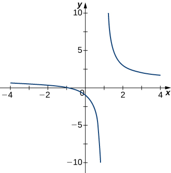
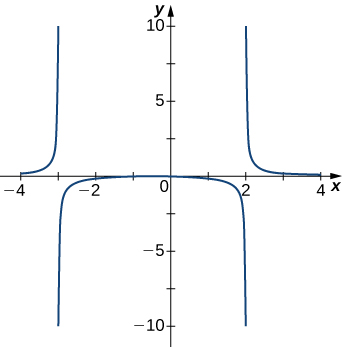
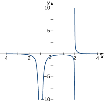
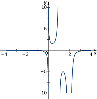
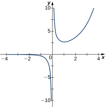
For the following exercises, examine the graphs. Identify where the vertical asymptotes are located.

The function graphed decreases very rapidly as it approaches x = 1 from the left, and on the other side of x = 1, it seems to start near infinity and then decrease rapidly.

Show Solution

The function graphed increases very rapidly as it approaches x = −3 from the left, and on the other side of x = −3, it seems to start near negative infinity and then increase rapidly to form a sort of U shape that is pointing down, with the other side of the U being at x = 2. On the other side of x = 2, the graph seems to start near infinity and then decrease rapidly.

The function graphed decreases very rapidly as it approaches x = −1 from the left, and on the other side of x = −1, it seems to start near negative infinity and then increase rapidly to form a sort of U shape that is pointing down, with the other side of the U being at x = 2. On the other side of x = 2, the graph seems to start near infinity and then decrease rapidly.

Show Solution

The function graphed decreases very rapidly as it approaches x = 0 from the left, and on the other side of x = 0, it seems to start near infinity and then decrease rapidly to form a sort of U shape that is pointing up, with the other side of the U being at x = 1. On the other side of x = 1, there is another U shape pointing down, with its other side being at x = 2. On the other side of x = 2, the graph seems to start near negative infinity and then increase rapidly.

Show Solution

For the following functions [latex]f(x)[/latex], determine whether there is an asymptote at [latex]x=a[/latex]. Justify your answer without graphing on a calculator.

6. [latex]f(x)=\frac{x+1}{x^2+5x+4}, \, a=-1[/latex]

7. [latex]f(x)=\frac{x}{x-2}, \, a=2[/latex]

Show Solution

8. [latex]f(x)=(x+2)^{3/2}, \, a=-2[/latex]

9. [latex]f(x)=(x-1)^{-1/3}, \, a=1[/latex]

Show Solution

10. [latex]f(x)=1+x^{-2/5}, \, a=1[/latex]

For the following exercises, evaluate the limit.

11. [latex]\underset{x\to \infty }{\lim}\frac{1}{3x+6}[/latex]

Show Solution

12. [latex]\underset{x\to \infty }{\lim}\frac{2x-5}{4x}[/latex]

13. [latex]\underset{x\to \infty }{\lim}\frac{x^2-2x+5}{x+2}[/latex]

Show Solution

14. [latex]\underset{x\to −\infty }{\lim}\frac{3x^3-2x}{x^2+2x+8}[/latex]

15. [latex]\underset{x\to −\infty }{\lim}\frac{x^4-4x^3+1}{2-2x^2-7x^4}[/latex]

Show Solution

16. [latex]\underset{x\to \infty }{\lim}\frac{3x}{\sqrt{x^2+1}}[/latex]

17. [latex]\underset{x\to −\infty }{\lim}\frac{\sqrt{4x^2-1}}{x+2}[/latex]

Show Solution

18. [latex]\underset{x\to \infty }{\lim}\frac{4x}{\sqrt{x^2-1}}[/latex]

19. [latex]\underset{x\to −\infty }{\lim}\frac{4x}{\sqrt{x^2-1}}[/latex]

Show Solution

20. [latex]\underset{x\to \infty }{\lim}\frac{2\sqrt{x}}{x-\sqrt{x}+1}[/latex]

For the following exercises, find the horizontal and vertical asymptotes.

21. [latex]f(x)=x-\frac{9}{x}[/latex]

Show Solution

22. [latex]f(x)=\frac{1}{1-x^2}[/latex]

23. [latex]f(x)=\frac{x^3}{4-x^2}[/latex]

Show Solution

24. [latex]f(x)=\frac{x^2+3}{x^2+1}[/latex]

25. [latex]f(x)= \sin (x) \sin (2x)[/latex]

Show Solution

26. [latex]f(x)= \cos x+ \cos (3x)+ \cos (5x)[/latex]

27. [latex]f(x)=\frac{x \sin (x)}{x^2-1}[/latex]

Show Solution

[latex]f(x)=\frac{x}{ \sin (x)}[/latex]

28. [latex]f(x)=\frac{1}{x^3+x^2}[/latex]

Show Solution

29. [latex]f(x)=\frac{1}{x-1}-2x[/latex]

30. [latex]f(x)=\frac{x^3+1}{x^3-1}[/latex]

Show Solution

31. [latex]f(x)=\frac{ \sin x+ \cos x}{ \sin x- \cos x}[/latex]

32. [latex]f(x)=x- \sin x[/latex]

Show Solution

33. [latex]f(x)=\frac{1}{x}-\sqrt{x}[/latex]

For the following exercises, construct a function [latex]f(x)[/latex] that has the given asymptotes.

34. [latex]x=1[/latex] and [latex]y=2[/latex]

Show Solution

35. [latex]x=1[/latex] and [latex]y=0[/latex]

36. [latex]y=4[/latex] and [latex]x=-1[/latex]

Show Solution

37. [latex]x=0[/latex]

For the following exercises, graph the function on a graphing calculator on the window [latex]x=[-5,5][/latex] and estimate the horizontal asymptote or limit. Then, calculate the actual horizontal asymptote or limit.

38. [T] [latex]f(x)=\frac{1}{x+10}[/latex]

Show Solution

39. [T] [latex]f(x)=\frac{x+1}{x^2+7x+6}[/latex]

40. [T] [latex]\underset{x\to −\infty }{\lim} x^2+10x+25[/latex]

Show Solution

41. [T] [latex]\underset{x\to −\infty }{\lim}\frac{x+2}{x^2+7x+6}[/latex]

42. [T] [latex]\underset{x\to \infty }{\lim}\frac{3x+2}{x+5}[/latex]

Show Solution

For the following exercises, draw a graph of the functions without using a calculator. Be sure to notice all important features of the graph: local maxima and minima, inflection points, and asymptotic behavior.

43. [latex]y=3x^2+2x+4[/latex]

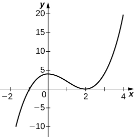
44. [latex]y=x^3-3x^2+4[/latex]

Show Solution

45. [latex]y=\frac{2x+1}{x^2+6x+5}[/latex]

46. [latex]y=\frac{x^3+4x^2+3x}{3x+9}[/latex]

Show Solution

47. [latex]y=\frac{x^2+x-2}{x^2-3x-4}[/latex]

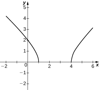
48. [latex]y=\sqrt{x^2-5x+4}[/latex]

Show Solution

49. [latex]y=2x\sqrt{16-x^2}[/latex]

50. [latex]y=\frac{ \cos x}{x}[/latex], on [latex]x=[-2\pi ,2\pi][/latex]

Show Solution

51. [latex]y=e^x-x^3[/latex]

52. [latex]y=x \tan x, \, x=[−\pi ,\pi][/latex]

Show Solution

53. [latex]y=x \ln (x), \, x>0[/latex]

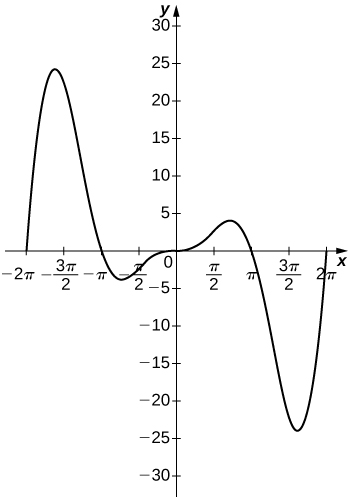
54. [latex]y=x^2 \sin (x), \, x=[-2\pi ,2\pi][/latex]

Show Solution

55. For [latex]f(x)=\frac{P(x)}{Q(x)}[/latex] to have an asymptote at [latex]y=2[/latex] then the polynomials [latex]P(x)[/latex] and [latex]Q(x)[/latex] must have what relation?

56. For [latex]f(x)=\frac{P(x)}{Q(x)}[/latex] to have an asymptote at [latex]x=0[/latex], then the polynomials [latex]P(x)[/latex] and [latex]Q(x)[/latex] must have what relation?

Show Solution

57. If [latex]f^{\prime}(x)[/latex] has asymptotes at [latex]y=3[/latex] and [latex]x=1[/latex], then [latex]f(x)[/latex] has what asymptotes?

58. Both [latex]f(x)=\frac{1}{x-1}[/latex] and [latex]g(x)=\frac{1}{(x-1)^2}[/latex] have asymptotes at [latex]x=1[/latex] and [latex]y=0[/latex]. What is the most obvious difference between these two functions?

Show Solution

59. True or false: Every ratio of polynomials has vertical asymptotes.

Glossary

end behavior: the behavior of a function as [latex]x\to \infty [/latex] and [latex]x\to −\infty [/latex]

horizontal asymptote: if [latex]\underset{x\to \infty }{\lim}f(x)=L[/latex] or [latex]\underset{x\to −\infty }{\lim}f(x)=L[/latex], then [latex]y=L[/latex] is a horizontal asymptote of [latex]f[/latex]

infinite limit at infinity: a function that becomes arbitrarily large as [latex]x[/latex] becomes large

limit at infinity: the limiting value, if it exists, of a function as [latex]x\to \infty [/latex] or [latex]x\to −\infty [/latex]

oblique asymptote: the line [latex]y=mx+b[/latex] if [latex]f(x)[/latex] approaches it as [latex]x\to \infty [/latex] or [latex]x\to −\infty [/latex]

4. Applications of Derivatives

4.6 Limits at Infinity and Asymptotes

Learning Objectives

Limits at Infinity

Limits at Infinity and Horizontal Asymptotes

Definition

Definition

Computing Limits at Infinity

Hint

Infinite Limits at Infinity

Definition

Formal Definitions

Definition

A Finite Limit at Infinity Example

Hint

Definition

An Infinite Limit at Infinity

Hint

End Behavior

End Behavior for Polynomial Functions

Limits at Infinity for Power Functions

Hint

End Behavior for Algebraic Functions

Determining End Behavior for Rational Functions

Hint

Determining End Behavior for a Function Involving a Radical

Hint

Determining End Behavior for Transcendental Functions

Determining End Behavior for a Transcendental Function

Hint

Guidelines for Drawing the Graph of a Function

Problem-Solving Strategy: Drawing the Graph of a Function

Sketching a Graph of a Polynomial

Hint

Sketching a Rational Function

Hint

Sketching a Rational Function with an Oblique Asymptote

Hint

Sketching the Graph of a Function with a Cusp

Hint

Key Concepts

Glossary