Learning Objectives
- Explain how the sign of the first derivative affects the shape of a function’s graph.
- State the first derivative test for critical points.
- Use concavity and inflection points to explain how the sign of the second derivative affects the shape of a function’s graph.
- Explain the concavity test for a function over an open interval.
- Explain the relationship between a function and its first and second derivatives.
- State the second derivative test for local extrema.
Earlier in this chapter we stated that if a function [latex]f[/latex] has a local extremum at a point [latex]c[/latex], then [latex]c[/latex] must be a critical point of [latex]f[/latex]. However, a function is not guaranteed to have a local extremum at a critical point. For example, [latex]f(x)=x^3[/latex] has a critical point at [latex]x=0[/latex] since [latex]f^{\prime}(x)=3x^2[/latex] is zero at [latex]x=0[/latex], but [latex]f[/latex] does not have a local extremum at [latex]x=0[/latex]. Using the results from the previous section, we are now able to determine whether a critical point of a function actually corresponds to a local extreme value. In this section, we also see how the second derivative provides information about the shape of a graph by describing whether the graph of a function curves upward or curves downward.
The First Derivative Test
Corollary 3 of the Mean Value Theorem showed that if the derivative of a function is positive over an interval [latex]I[/latex] then the function is increasing over [latex]I[/latex]. On the other hand, if the derivative of the function is negative over an interval [latex]I[/latex], then the function is decreasing over [latex]I[/latex] as shown in the following figure.
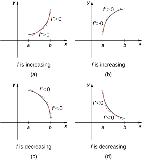
Figure 1. Both functions are increasing over the interval [latex](a,b)[/latex]. At each point [latex]x[/latex], the derivative [latex]f^{\prime}(x)>0[/latex]. Both functions are decreasing over the interval [latex](a,b)[/latex]. At each point [latex]x[/latex], the derivative [latex]f^{\prime}(x)<0[/latex].
A continuous function [latex]f[/latex] has a local maximum at point [latex]c[/latex] if and only if [latex]f[/latex] switches from increasing to decreasing at point [latex]c[/latex]. Similarly, [latex]f[/latex] has a local minimum at [latex]c[/latex] if and only if [latex]f[/latex] switches from decreasing to increasing at [latex]c[/latex]. If [latex]f[/latex] is a continuous function over an interval [latex]I[/latex] containing [latex]c[/latex] and differentiable over [latex]I[/latex], except possibly at [latex]c[/latex], the only way [latex]f[/latex] can switch from increasing to decreasing (or vice versa) at point [latex]c[/latex] is if [latex]{f}^{\prime }[/latex] changes sign as [latex]x[/latex] increases through [latex]c.[/latex] If [latex]f[/latex] is differentiable at [latex]c,[/latex] the only way that [latex]{f}^{\prime }.[/latex] can change sign as [latex]x[/latex] increases through [latex]c[/latex] is if [latex]f^{\prime}(c)=0[/latex]. Therefore, for a function [latex]f[/latex] that is continuous over an interval [latex]I[/latex] containing [latex]c[/latex] and differentiable over [latex]I[/latex], except possibly at [latex]c[/latex], the only way [latex]f[/latex] can switch from increasing to decreasing (or vice versa) is if [latex]f^{\prime}(c)=0[/latex] or [latex]f^{\prime}(c)[/latex] is undefined. Consequently, to locate local extrema for a function [latex]f[/latex], we look for points [latex]c[/latex] in the domain of [latex]f[/latex] such that [latex]f^{\prime}(c)=0[/latex] or [latex]f^{\prime}(c)[/latex] is undefined. Recall that such points are called critical points of [latex]f[/latex].
Note that [latex]f[/latex] need not have a local extrema at a critical point. The critical points are candidates for local extrema only. In (Figure), we show that if a continuous function [latex]f[/latex] has a local extremum, it must occur at a critical point, but a function may not have a local extremum at a critical point. We show that if [latex]f[/latex] has a local extremum at a critical point, then the sign of [latex]f^{\prime}[/latex] switches as [latex]x[/latex] increases through that point.
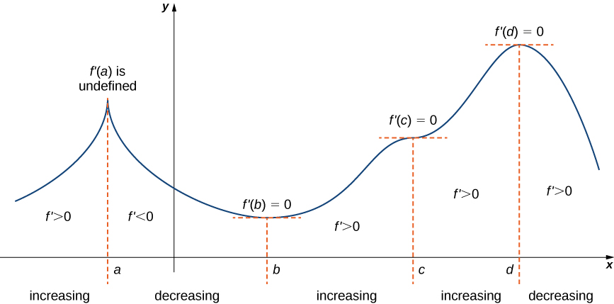
Figure 2. The function [latex]f[/latex] has four critical points: [latex]a,b,c[/latex], and [latex]d[/latex]. The function [latex]f[/latex] has local maxima at [latex]a[/latex] and [latex]d[/latex], and a local minimum at [latex]b[/latex]. The function [latex]f[/latex] does not have a local extremum at [latex]c[/latex]. The sign of [latex]f^{\prime}[/latex] changes at all local extrema.
Using (Figure), we summarize the main results regarding local extrema.
- If a continuous function [latex]f[/latex] has a local extremum, it must occur at a critical point [latex]c[/latex].
- The function has a local extremum at the critical point [latex]c[/latex] if and only if the derivative [latex]f^{\prime}[/latex] switches sign as [latex]x[/latex] increases through [latex]c[/latex].
- Therefore, to test whether a function has a local extremum at a critical point [latex]c[/latex], we must determine the sign of [latex]f^{\prime}(x)[/latex] to the left and right of [latex]c[/latex].
This result is known as the first derivative test.
First Derivative Test
Suppose that [latex]f[/latex] is a continuous function over an interval [latex]I[/latex] containing a critical point [latex]c[/latex]. If [latex]f[/latex] is differentiable over [latex]I[/latex], except possibly at point [latex]c[/latex], then [latex]f(c)[/latex] satisfies one of the following descriptions:
- If [latex]f^{\prime}[/latex] changes sign from positive when [latex]x
- If [latex]f^{\prime}[/latex] changes sign from negative when [latex]x
- If [latex]f^{\prime}[/latex] has the same sign for [latex]x
We can summarize the first derivative test as a strategy for locating local extrema.
Problem-Solving Strategy: Using the First Derivative Test
Consider a function [latex]f[/latex] that is continuous over an interval [latex]I[/latex].
- Find all critical points of [latex]f[/latex] and divide the interval [latex]I[/latex] into smaller intervals using the critical points as endpoints.
- Analyze the sign of [latex]f^{\prime}[/latex] in each of the subintervals. If [latex]f^{\prime}[/latex] is continuous over a given subinterval (which is typically the case), then the sign of [latex]f^{\prime}[/latex] in that subinterval does not change and, therefore, can be determined by choosing an arbitrary test point [latex]x[/latex] in that subinterval and by evaluating the sign of [latex]f^{\prime}[/latex] at that test point. Use the sign analysis to determine whether [latex]f[/latex] is increasing or decreasing over that interval.
- Use (Figure) and the results of step 2 to determine whether [latex]f[/latex] has a local maximum, a local minimum, or neither at each of the critical points.
Now let’s look at how to use this strategy to locate all local extrema for particular functions.
Using the First Derivative Test to Find Local Extrema
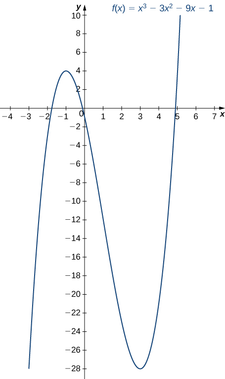
Use the first derivative test to find the location of all local extrema for [latex]f(x)=x^3-3x^2-9x-1[/latex]. Use a graphing utility to confirm your results.
Use the first derivative test to locate all local extrema for [latex]f(x)=−x^3+\frac{3}{2}x^2+18x[/latex].
Using the First Derivative Test
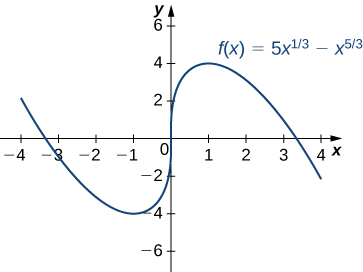
Use the first derivative test to find the location of all local extrema for [latex]f(x)=5x^{1/3}-x^{5/3}[/latex]. Use a graphing utility to confirm your results.
Use the first derivative test to find all local extrema for [latex]f(x)=\sqrt[3]{x-1}[/latex].
Hint
The only critical point of [latex]f[/latex] is [latex]x=1[/latex].
Concavity and Points of Inflection
We now know how to determine where a function is increasing or decreasing. However, there is another issue to consider regarding the shape of the graph of a function. If the graph curves, does it curve upward or curve downward? This notion is called the concavity of the function.
(Figure)(a) shows a function [latex]f[/latex] with a graph that curves upward. As [latex]x[/latex] increases, the slope of the tangent line increases. Thus, since the derivative increases as [latex]x[/latex] increases, [latex]f^{\prime}[/latex] is an increasing function. We say this function [latex]f[/latex] is concave up. (Figure)(b) shows a function [latex]f[/latex] that curves downward. As [latex]x[/latex] increases, the slope of the tangent line decreases. Since the derivative decreases as [latex]x[/latex] increases, [latex]f^{\prime}[/latex] is a decreasing function. We say this function [latex]f[/latex] is concave down.
Definition
Let [latex]f[/latex] be a function that is differentiable over an open interval [latex]I[/latex]. If [latex]f^{\prime}[/latex] is increasing over [latex]I[/latex], we say [latex]f[/latex] is concave up over [latex]I[/latex]. If [latex]f^{\prime}[/latex] is decreasing over [latex]I[/latex], we say [latex]f[/latex] is concave down over [latex]I[/latex].
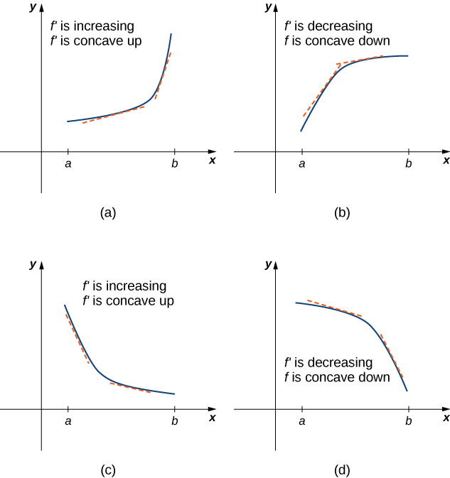
Figure 5. (a), (c) Since [latex]f^{\prime}[/latex] is increasing over the interval [latex](a,b)[/latex], we say [latex]f[/latex] is concave up over [latex](a,b)[/latex]. (b), (d) Since [latex]f^{\prime}[/latex] is decreasing over the interval [latex](a,b)[/latex], we say [latex]f[/latex] is concave down over [latex](a,b)[/latex].
In general, without having the graph of a function [latex]f[/latex], how can we determine its concavity? By definition, a function [latex]f[/latex] is concave up if [latex]f^{\prime}[/latex] is increasing. From Corollary 3, we know that if [latex]f^{\prime}[/latex] is a differentiable function, then [latex]f^{\prime}[/latex] is increasing if its derivative [latex]f^{\prime \prime}(x)>0[/latex]. Therefore, a function [latex]f[/latex] that is twice differentiable is concave up when [latex]f^{\prime \prime}(x)>0[/latex]. Similarly, a function [latex]f[/latex] is concave down if [latex]f^{\prime}[/latex] is decreasing. We know that a differentiable function [latex]f^{\prime}[/latex] is decreasing if its derivative [latex]f^{\prime \prime}(x)<0[/latex]. Therefore, a twice-differentiable function [latex]f[/latex] is concave down when [latex]f^{\prime \prime}(x)<0[/latex]. Applying this logic is known as the concavity test.
Test for Concavity
Let [latex]f[/latex] be a function that is twice differentiable over an interval [latex]I[/latex].
- If [latex]f^{\prime \prime}(x)>0[/latex] for all [latex]x \in I[/latex], then [latex]f[/latex] is concave up over [latex]I[/latex].
- If [latex]f^{\prime \prime}(x)<0[/latex] for all [latex]x \in I[/latex], then [latex]f[/latex] is concave down over [latex]I[/latex].
We conclude that we can determine the concavity of a function [latex]f[/latex] by looking at the second derivative of [latex]f[/latex]. In addition, we observe that a function [latex]f[/latex] can switch concavity ((Figure)). However, a continuous function can switch concavity only at a point [latex]x[/latex] if [latex]f^{\prime \prime}(x)=0[/latex] or [latex]f^{\prime \prime}(x)[/latex] is undefined. Consequently, to determine the intervals where a function [latex]f[/latex] is concave up and concave down, we look for those values of [latex]x[/latex] where [latex]f^{\prime \prime}(x)=0[/latex] or [latex]f^{\prime \prime}(x)[/latex] is undefined. When we have determined these points, we divide the domain of [latex]f[/latex] into smaller intervals and determine the sign of [latex]f^{\prime \prime}[/latex] over each of these smaller intervals. If [latex]f^{\prime \prime}[/latex] changes sign as we pass through a point [latex]x[/latex], then [latex]f[/latex] changes concavity. It is important to remember that a function [latex]f[/latex] may not change concavity at a point [latex]x[/latex] even if [latex]f^{\prime \prime}(x)=0[/latex] or [latex]f^{\prime \prime}(x)[/latex] is undefined. If, however, [latex]f[/latex] does change concavity at a point [latex]a[/latex] and [latex]f[/latex] is continuous at [latex]a[/latex], we say the point [latex](a,f(a))[/latex] is an inflection point of [latex]f[/latex].
Definition
If [latex]f[/latex] is continuous at [latex]a[/latex] and [latex]f[/latex] changes concavity at [latex]a[/latex], the point [latex](a,f(a))[/latex] is an inflection point of [latex]f[/latex].
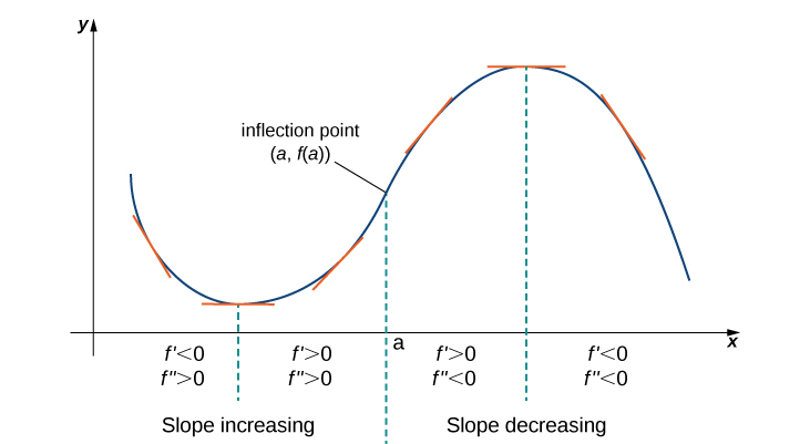
Figure 6. Since [latex]f^{\prime \prime}(x)>0[/latex] for [latex]x<a[/latex], the function [latex]f[/latex] is concave up over the interval [latex](−\infty,a)[/latex]. Since [latex]f^{\prime \prime}(x)<0[/latex] for [latex]x>a[/latex], the function [latex]f[/latex] is concave down over the interval [latex](a,\infty)[/latex]. The point [latex](a,f(a))[/latex] is an inflection point of [latex]f[/latex].
Testing for Concavity
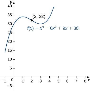
For the function [latex]f(x)=x^3-6x^2+9x+30[/latex], determine all intervals where [latex]f[/latex] is concave up and all intervals where [latex]f[/latex] is concave down. List all inflection points for [latex]f[/latex]. Use a graphing utility to confirm your results.
For [latex]f(x)=−x^3+\frac{3}{2}x^2+18x[/latex], find all intervals where [latex]f[/latex] is concave up and all intervals where [latex]f[/latex] is concave down.
Hint
Find where [latex]f^{\prime \prime}(x)=0[/latex].
We now summarize, in (Figure), the information that the first and second derivatives of a function [latex]f[/latex] provide about the graph of [latex]f[/latex], and illustrate this information in (Figure).
| Sign of [latex]f^{\prime}[/latex] | Sign of [latex]f^{\prime \prime}[/latex] | Is [latex]f[/latex] increasing or decreasing? | Concavity |
|---|---|---|---|
| Positive | Positive | Increasing | Concave up |
| Positive | Negative | Increasing | Concave down |
| Negative | Positive | Decreasing | Concave up |
| Negative | Negative | Decreasing | Concave down |
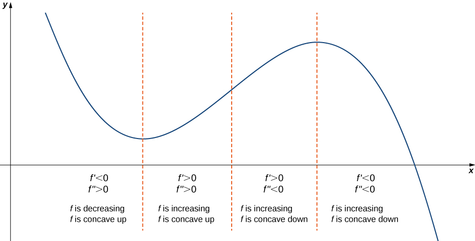
Figure 8. Consider a twice-differentiable function [latex]f[/latex] over an open interval [latex]I[/latex]. If [latex]f^{\prime}(x)>0[/latex] for all [latex]x \in I[/latex], the function is increasing over [latex]I[/latex]. If [latex]f^{\prime}(x)<0[/latex] for all [latex]x \in I[/latex], the function is decreasing over [latex]I[/latex]. If [latex]f^{\prime \prime}(x)>0[/latex] for all [latex]x \in I[/latex], the function is concave up. If [latex]f^{\prime \prime}(x)<0[/latex] for all [latex]x \in I[/latex], the function is concave down on [latex]I[/latex].
The Second Derivative Test
The first derivative test provides an analytical tool for finding local extrema, but the second derivative can also be used to locate extreme values. Using the second derivative can sometimes be a simpler method than using the first derivative.
We know that if a continuous function has a local extrema, it must occur at a critical point. However, a function need not have a local extrema at a critical point. Here we examine how the second derivative test can be used to determine whether a function has a local extremum at a critical point. Let [latex]f[/latex] be a twice-differentiable function such that [latex]f^{\prime}(a)=0[/latex] and [latex]f^{\prime \prime}[/latex] is continuous over an open interval [latex]I[/latex] containing [latex]a[/latex]. Suppose [latex]f^{\prime \prime}(a)<0[/latex]. Since [latex]f^{\prime \prime}[/latex] is continuous over [latex]I[/latex], [latex]f^{\prime \prime}(x)<0[/latex] for all [latex]x \in I[/latex] ((Figure)). Then, by Corollary 3, [latex]f^{\prime}[/latex] is a decreasing function over [latex]I[/latex]. Since [latex]f^{\prime}(a)=0[/latex], we conclude that for all [latex]x \in I, \, f^{\prime}(x)>0[/latex] if [latex]x
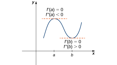
Figure 9. Consider a twice-differentiable function [latex]f[/latex] such that [latex]f^{\prime \prime}[/latex] is continuous. Since [latex]f^{\prime}(a)=0[/latex] and [latex]f^{\prime \prime}(a)<0[/latex], there is an interval [latex]I[/latex] containing [latex]a[/latex] such that for all [latex]x[/latex] in [latex]I[/latex], [latex]f[/latex] is increasing if [latex]x<a[/latex] and [latex]f[/latex] is decreasing if [latex]x>a[/latex]. As a result, [latex]f[/latex] has a local maximum at [latex]x=a[/latex]. Since [latex]f^{\prime}(b)=0[/latex] and [latex]f^{\prime \prime}(b)>0[/latex], there is an interval [latex]I[/latex] containing [latex]b[/latex] such that for all [latex]x[/latex] in [latex]I[/latex], [latex]f[/latex] is decreasing if [latex]x<b[/latex] and [latex]f[/latex] is increasing if [latex]x>b[/latex]. As a result, [latex]f[/latex] has a local minimum at [latex]x=b[/latex].
Second Derivative Test
Suppose [latex]f^{\prime}(c)=0, \, f^{\prime \prime}[/latex] is continuous over an interval containing [latex]c[/latex].
- If [latex]f^{\prime \prime}(c)>0[/latex], then [latex]f[/latex] has a local minimum at [latex]c[/latex].
- If [latex]f^{\prime \prime}(c)<0[/latex], then [latex]f[/latex] has a local maximum at [latex]c[/latex].
- If [latex]f^{\prime \prime}(c)=0[/latex], then the test is inconclusive.
Note that for case iii. when [latex]f^{\prime \prime}(c)=0[/latex], then [latex]f[/latex] may have a local maximum, local minimum, or neither at [latex]c[/latex]. For example, the functions [latex]f(x)=x^3[/latex], [latex]f(x)=x^4[/latex], and [latex]f(x)=−x^4[/latex] all have critical points at [latex]x=0[/latex]. In each case, the second derivative is zero at [latex]x=0[/latex]. However, the function [latex]f(x)=x^4[/latex] has a local minimum at [latex]x=0[/latex] whereas the function [latex]f(x)=−x^4[/latex] has a local maximum at [latex]x=0[/latex] and the function [latex]f(x)=x^3[/latex] does not have a local extremum at [latex]x=0[/latex].
Let’s now look at how to use the second derivative test to determine whether [latex]f[/latex] has a local maximum or local minimum at a critical point [latex]c[/latex] where [latex]f^{\prime}(c)=0[/latex].
Using the Second Derivative Test
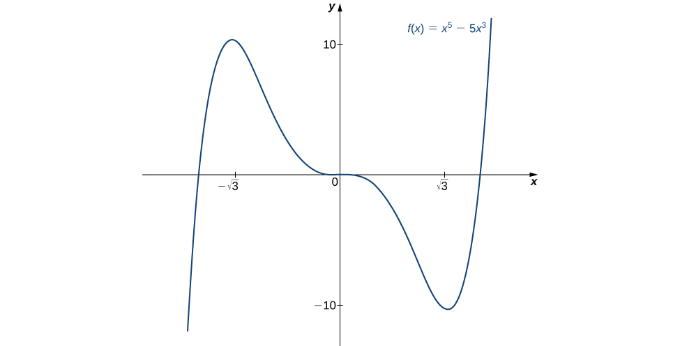
Use the second derivative to find the location of all local extrema for [latex]f(x)=x^5-5x^3[/latex].
Consider the function [latex]f(x)=x^3-(\frac{3}{2})x^2-18x[/latex]. The points [latex]c=3,-2[/latex] satisfy [latex]f^{\prime}(c)=0[/latex]. Use the second derivative test to determine whether [latex]f[/latex] has a local maximum or local minimum at those points.
Hint
[latex]f^{\prime \prime}(x)=6x-3[/latex]
We have now developed the tools we need to determine where a function is increasing and decreasing, as well as acquired an understanding of the basic shape of the graph. In the next section we discuss what happens to a function as [latex]x \to \pm \infty[/latex]. At that point, we have enough tools to provide accurate graphs of a large variety of functions.
Key Concepts
- If [latex]c[/latex] is a critical point of [latex]f[/latex] and [latex]f^{\prime}(x)>0[/latex] for [latex]x
- If [latex]c[/latex] is a critical point of [latex]f[/latex] and [latex]f^{\prime}(x)<0[/latex] for [latex]x
- If [latex]f^{\prime \prime}(x)>0[/latex] over an interval [latex]I[/latex], then [latex]f[/latex] is concave up over [latex]I[/latex].
- If [latex]f^{\prime \prime}(x)<0[/latex] over an interval [latex]I[/latex], then [latex]f[/latex] is concave down over [latex]I[/latex].
- If [latex]f^{\prime}(c)=0[/latex] and [latex]f^{\prime \prime}(c)>0[/latex], then [latex]f[/latex] has a local minimum at [latex]c[/latex].
- If [latex]f^{\prime}(c)=0[/latex] and [latex]f^{\prime \prime}(c)<0[/latex], then [latex]f[/latex] has a local maximum at [latex]c[/latex].
- If [latex]f^{\prime}(c)=0[/latex] and [latex]f^{\prime \prime}(c)=0[/latex], then evaluate [latex]f^{\prime}(x)[/latex] at a test point [latex]x[/latex] to the left of [latex]c[/latex] and a test point [latex]x[/latex] to the right of [latex]c[/latex], to determine whether [latex]f[/latex] has a local extremum at [latex]c[/latex].
1. If [latex]c[/latex] is a critical point of [latex]f(x)[/latex], when is there no local maximum or minimum at [latex]c[/latex]? Explain.
2. For the function [latex]y=x^3[/latex], is [latex]x=0[/latex] both an inflection point and a local maximum/minimum?
3. For the function [latex]y=x^3[/latex], is [latex]x=0[/latex] an inflection point?
4. Is it possible for a point [latex]c[/latex] to be both an inflection point and a local extrema of a twice differentiable function?
5. Why do you need continuity for the first derivative test? Come up with an example.
6. Explain whether a concave-down function has to cross [latex]y=0[/latex] for some value of [latex]x[/latex].
7. Explain whether a polynomial of degree 2 can have an inflection point.
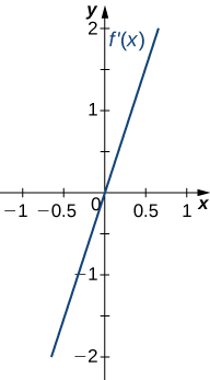
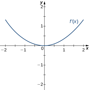
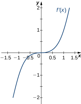
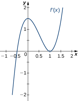
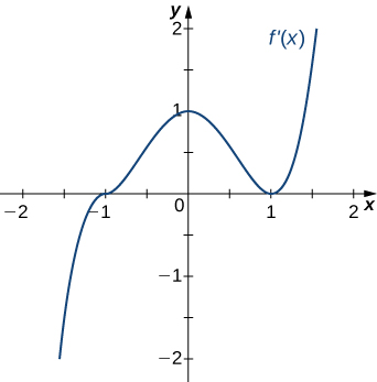
For the following exercises, analyze the graphs of [latex]f^{\prime}[/latex], then list all intervals where [latex]f[/latex] is increasing or decreasing.
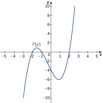
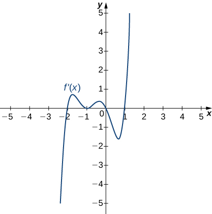
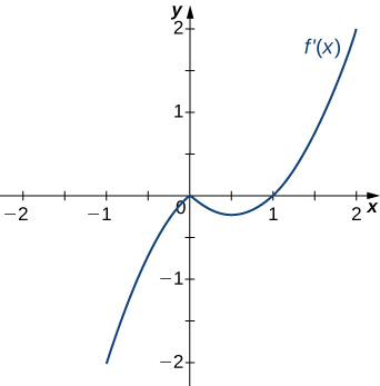
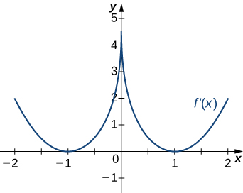
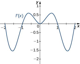
For the following exercises, analyze the graphs of [latex]f^{\prime}[/latex], then list
- all intervals where [latex]f[/latex] is increasing and decreasing and
- where the minima and maxima are located.
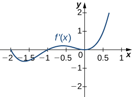
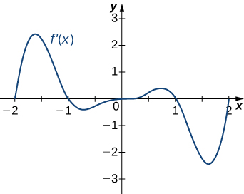
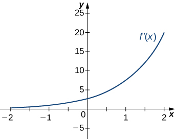
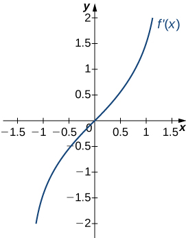
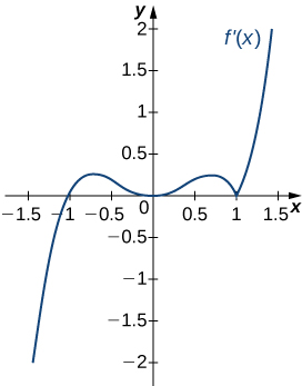
For the following exercises, analyze the graphs of [latex]f^{\prime}[/latex], then list all inflection points and intervals [latex]f[/latex] that are concave up and concave down.
For the following exercises, draw a graph that satisfies the given specifications for the domain [latex]x=[-3,3][/latex]. The function does not have to be continuous or differentiable.
23. [latex]f(x)>0, \, f^{\prime}(x)>0[/latex] over [latex]x>1, \, -3
24. [latex]f^{\prime}(x)>0[/latex] over [latex]x>2, \, -3
25. [latex]f^{\prime \prime}(x)<0[/latex] over [latex]-1
26. There is a local maximum at [latex]x=2[/latex], local minimum at [latex]x=1[/latex], and the graph is neither concave up nor concave down.
27. There are local maxima at [latex]x=\pm 1[/latex], the function is concave up for all [latex]x[/latex], and the function remains positive for all [latex]x[/latex].
For the following exercises, determine
- intervals where [latex]f[/latex] is increasing or decreasing and
- local minima and maxima of [latex]f[/latex].
28. [latex]f(x)= \sin x+ \sin^3 x[/latex] over [latex]−\pi
29. [latex]f(x)=x^2 + \cos x[/latex]
For the following exercises, determine a. intervals where [latex]f[/latex] is concave up or concave down, and b. the inflection points of [latex]f[/latex].
30. [latex]f(x)=x^3-4x^2+x+2[/latex]
For the following exercises, determine
- intervals where [latex]f[/latex] is increasing or decreasing,
- local minima and maxima of [latex]f[/latex],
- intervals where [latex]f[/latex] is concave up and concave down, and
- the inflection points of [latex]f[/latex].
31. [latex]f(x)=x^2-6x[/latex]
32. [latex]f(x)=x^3-6x^2[/latex]
33. [latex]f(x)=x^4-6x^3[/latex]
34. [latex]f(x)=x^{11}-6x^{10}[/latex]
35. [latex]f(x)=x+x^2-x^3[/latex]
36. [latex]f(x)=x^2+x+1[/latex]
37. [latex]f(x)=x^3+x^4[/latex]
For the following exercises, determine
- intervals where [latex]f[/latex] is increasing or decreasing,
- local minima and maxima of [latex]f[/latex],
- intervals where [latex]f[/latex] is concave up and concave down, and
- the inflection points of [latex]f[/latex]. Sketch the curve, then use a calculator to compare your answer. If you cannot determine the exact answer analytically, use a calculator.
38. [T] [latex]f(x)= \sin (\pi x)- \cos (\pi x)[/latex] over [latex]x=[-1,1][/latex]
39. [T] [latex]f(x)=x + \sin (2x)[/latex] over [latex]x=[-\frac{\pi }{2},\frac{\pi }{2}][/latex]
40. [T] [latex]f(x)= \sin x+ \tan x[/latex] over [latex](-\frac{\pi }{2},\frac{\pi }{2})[/latex]
41. [T] [latex]f(x)=(x-2)^2 (x-4)^2[/latex]
42. [T] [latex]f(x)=\frac{1}{1-x}, \, x \ne 1[/latex]
43. [T] [latex]f(x)=\frac{\sin x}{x}[/latex] over [latex]x=[-2\pi ,0) \cup (0,2\pi][/latex]
44. [latex]f(x)= \sin x e^x[/latex] over [latex]x=[−\pi ,\pi][/latex]
45. [latex]f(x)=\ln x \sqrt{x}, \, x>0[/latex]
46. [latex]f(x)=\frac{1}{4}\sqrt{x}+\frac{1}{x}, \, x>0[/latex]
47. [latex]f(x)=\frac{e^x}{x}, \, x\ne 0[/latex]
For the following exercises, interpret the sentences in terms of [latex]f, \, f^{\prime}[/latex], and [latex]f^{\prime \prime}[/latex].
48. The population is growing more slowly. Here [latex]f[/latex] is the population.
49. A bike accelerates faster, but a car goes faster. Here [latex]f[/latex] represents the Bike’s position minus the Car’s position.
50. The airplane lands smoothly. Here [latex]f[/latex] is the plane’s altitude.
51. Stock prices are at their peak. Here [latex]f[/latex] is the stock price.
52. The economy is picking up speed. Here [latex]f[/latex] is a measure of the economy, such as GDP.
For the following exercises, consider a third-degree polynomial [latex]f(x)[/latex], which has the properties [latex]f^{\prime}(1)=0, \, f^{\prime}(3)=0[/latex]. Determine whether the following statements are true or false. Justify your answer.
53. [latex]f(x)=0[/latex] for some [latex]1 \le x \le 3[/latex]
54. [latex]f^{\prime \prime}(x)=0[/latex] for some [latex]1 \le x \le 3[/latex]
55. There is no absolute maximum at [latex]x=3[/latex]
56. If [latex]f(x)[/latex] has three roots, then it has 1 inflection point.
57. If [latex]f(x)[/latex] has one inflection point, then it has three real roots.
Glossary
- concave down
- if [latex]f[/latex] is differentiable over an interval [latex]I[/latex] and [latex]f^{\prime}[/latex] is decreasing over [latex]I[/latex], then [latex]f[/latex] is concave down over [latex]I[/latex]
- concave up
- if [latex]f[/latex] is differentiable over an interval [latex]I[/latex] and [latex]f^{\prime}[/latex] is increasing over [latex]I[/latex], then [latex]f[/latex] is concave up over [latex]I[/latex]
- concavity
- the upward or downward curve of the graph of a function
- concavity test
- suppose [latex]f[/latex] is twice differentiable over an interval [latex]I[/latex]; if [latex]f^{\prime \prime}>0[/latex] over [latex]I[/latex], then [latex]f[/latex] is concave up over [latex]I[/latex]; if [latex]f^{\prime \prime}<0[/latex] over [latex]I[/latex], then [latex]f[/latex] is concave down over [latex]I[/latex]
- first derivative test
- let [latex]f[/latex] be a continuous function over an interval [latex]I[/latex] containing a critical point [latex]c[/latex] such that [latex]f[/latex] is differentiable over [latex]I[/latex] except possibly at [latex]c[/latex]; if [latex]f^{\prime}[/latex] changes sign from positive to negative as [latex]x[/latex] increases through [latex]c[/latex], then [latex]f[/latex] has a local maximum at [latex]c[/latex]; if [latex]f^{\prime}[/latex] changes sign from negative to positive as [latex]x[/latex] increases through [latex]c[/latex], then [latex]f[/latex] has a local minimum at [latex]c[/latex]; if [latex]f^{\prime}[/latex] does not change sign as [latex]x[/latex] increases through [latex]c[/latex], then [latex]f[/latex] does not have a local extremum at [latex]c[/latex]
- inflection point
- if [latex]f[/latex] is continuous at [latex]c[/latex] and [latex]f[/latex] changes concavity at [latex]c[/latex], the point [latex](c,f(c))[/latex] is an inflection point of [latex]f[/latex]
- second derivative test
- suppose [latex]f^{\prime}(c)=0[/latex] and [latex]f^{\prime \prime}[/latex] is continuous over an interval containing [latex]c[/latex]; if [latex]f^{\prime \prime}(c)>0[/latex], then [latex]f[/latex] has a local minimum at [latex]c[/latex]; if [latex]f^{\prime \prime}(c)<0[/latex], then [latex]f[/latex] has a local maximum at [latex]c[/latex]; if [latex]f^{\prime \prime}(c)=0[/latex], then the test is inconclusive
Candela Citations
- Calculus I. Provided by: OpenStax. Located at: http://cnx.org/contents/8b89d172-2927-466f-8661-01abc7ccdba4@2.89. License: CC BY-NC-SA: Attribution-NonCommercial-ShareAlike. License Terms: Download for free at http://cnx.org/contents/8b89d172-2927-466f-8661-01abc7ccdba4@2.89

Hint
Find all critical points of [latex]f[/latex] and determine the signs of [latex]f^{\prime}(x)[/latex] over particular intervals determined by the critical points.