Learning Objectives
- Explain the meaning of Rolle’s theorem.
- Describe the significance of the Mean Value Theorem.
- State three important consequences of the Mean Value Theorem.
The Mean Value Theorem is one of the most important theorems in calculus. We look at some of its implications at the end of this section. First, let’s start with a special case of the Mean Value Theorem, called Rolle’s theorem.
Rolle’s Theorem
Informally, Rolle’s theorem states that if the outputs of a differentiable function [latex]f[/latex] are equal at the endpoints of an interval, then there must be an interior point [latex]c[/latex] where [latex]f^{\prime}(c)=0[/latex]. (Figure) illustrates this theorem.
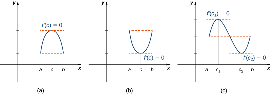
Figure 1. If a differentiable function f satisfies [latex]f(a)=f(b)[/latex], then its derivative must be zero at some point(s) between [latex]a[/latex] and [latex]b[/latex].
Rolle’s Theorem
Let [latex]f[/latex] be a continuous function over the closed interval [latex][a,b][/latex] and differentiable over the open interval [latex](a,b)[/latex] such that [latex]f(a)=f(b)[/latex]. There then exists at least one [latex]c \in (a,b)[/latex] such that [latex]f^{\prime}(c)=0[/latex].
Proof
Let [latex]k=f(a)=f(b)[/latex]. We consider three cases:
- [latex]f(x)=k[/latex] for all [latex]x \in (a,b)[/latex].
- There exists [latex]x \in (a,b)[/latex] such that [latex]f(x)>k[/latex].
- There exists [latex]x \in (a,b)[/latex] such that [latex]f(x)
Case 1: If [latex]f(x)=0[/latex] for all [latex]x \in (a,b)[/latex], then [latex]f^{\prime}(x)=0[/latex] for all [latex]x \in (a,b)[/latex].
Case 2: Since [latex]f[/latex] is a continuous function over the closed, bounded interval [latex][a,b][/latex], by the extreme value theorem, it has an absolute maximum. Also, since there is a point [latex]x \in (a,b)[/latex] such that [latex]f(x)>k[/latex], the absolute maximum is greater than [latex]k[/latex]. Therefore, the absolute maximum does not occur at either endpoint. As a result, the absolute maximum must occur at an interior point [latex]c \in (a,b)[/latex]. Because [latex]f[/latex] has a maximum at an interior point [latex]c[/latex], and [latex]f[/latex] is differentiable at [latex]c[/latex], by Fermat’s theorem, [latex]f^{\prime}(c)=0[/latex].
Case 3: The case when there exists a point [latex]x \in (a,b)[/latex] such that [latex]f(x) □ An important point about Rolle’s theorem is that the differentiability of the function [latex]f[/latex] is critical. If [latex]f[/latex] is not differentiable, even at a single point, the result may not hold. For example, the function [latex]f(x)=|x|-1[/latex] is continuous over [latex][-1,1][/latex] and [latex]f(-1)=0=f(1)[/latex], but [latex]f^{\prime}(c) \ne 0[/latex] for any [latex]c \in (-1,1)[/latex] as shown in the following figure. Figure 2. Since [latex]f(x)=|x|-1[/latex] is not differentiable at [latex]x=0[/latex], the conditions of Rolle’s theorem are not satisfied. In fact, the conclusion does not hold here; there is no [latex]c \in (-1,1)[/latex] such that [latex]f^{\prime}(c)=0[/latex]. Let’s now consider functions that satisfy the conditions of Rolle’s theorem and calculate explicitly the points [latex]c[/latex] where [latex]f^{\prime}(c)=0[/latex]. For each of the following functions, verify that the function satisfies the criteria stated in Rolle’s theorem and find all values [latex]c[/latex] in the given interval where [latex]f^{\prime}(c)=0[/latex]. Verify that the function [latex]f(x)=2x^2-8x+6[/latex] defined over the interval [latex][1,3][/latex] satisfies the conditions of Rolle’s theorem. Find all points [latex]c[/latex] guaranteed by Rolle’s theorem.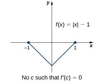
Using Rolle’s Theorem
The Mean Value Theorem and Its Meaning
Rolle’s theorem is a special case of the Mean Value Theorem. In Rolle’s theorem, we consider differentiable functions [latex]f[/latex] that are zero at the endpoints. The Mean Value Theorem generalizes Rolle’s theorem by considering functions that are not necessarily zero at the endpoints. Consequently, we can view the Mean Value Theorem as a slanted version of Rolle’s theorem ((Figure)). The Mean Value Theorem states that if [latex]f[/latex] is continuous over the closed interval [latex][a,b][/latex] and differentiable over the open interval [latex](a,b)[/latex], then there exists a point [latex]c \in (a,b)[/latex] such that the tangent line to the graph of [latex]f[/latex] at [latex]c[/latex] is parallel to the secant line connecting [latex](a,f(a))[/latex] and [latex](b,f(b))[/latex].
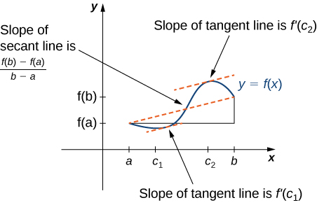
Figure 5. The Mean Value Theorem says that for a function that meets its conditions, at some point the tangent line has the same slope as the secant line between the ends. For this function, there are two values [latex]c_1[/latex] and [latex]c_2[/latex] such that the tangent line to [latex]f[/latex] at [latex]c_1[/latex] and [latex]c_2[/latex] has the same slope as the secant line.
Mean Value Theorem
Let [latex]f[/latex] be continuous over the closed interval [latex][a,b][/latex] and differentiable over the open interval [latex](a,b)[/latex]. Then, there exists at least one point [latex]c \in (a,b)[/latex] such that
Proof
The proof follows from Rolle’s theorem by introducing an appropriate function that satisfies the criteria of Rolle’s theorem. Consider the line connecting [latex](a,f(a))[/latex] and [latex](b,f(b))[/latex]. Since the slope of that line is
and the line passes through the point [latex](a,f(a))[/latex], the equation of that line can be written as
Let [latex]g(x)[/latex] denote the vertical difference between the point [latex](x,f(x))[/latex] and the point [latex](x,y)[/latex] on that line. Therefore,
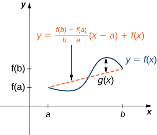
Figure 6. The value [latex]g(x)[/latex] is the vertical difference between the point [latex](x,f(x))[/latex] and the point [latex](x,y)[/latex] on the secant line connecting [latex](a,f(a))[/latex] and [latex](b,f(b)).[/latex]
Since the graph of [latex]f[/latex] intersects the secant line when [latex]x=a[/latex] and [latex]x=b[/latex], we see that [latex]g(a)=0=g(b)[/latex]. Since [latex]f[/latex] is a differentiable function over [latex](a,b)[/latex], [latex]g[/latex] is also a differentiable function over [latex](a,b)[/latex]. Furthermore, since [latex]f[/latex] is continuous over [latex][a,b][/latex], [latex]g[/latex] is also continuous over [latex][a,b][/latex]. Therefore, [latex]g[/latex] satisfies the criteria of Rolle’s theorem. Consequently, there exists a point [latex]c \in (a,b)[/latex] such that [latex]g^{\prime}(c)=0[/latex]. Since
we see that
Since [latex]g^{\prime}(c)=0[/latex], we conclude that
□
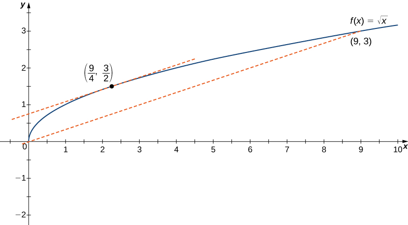
In the next example, we show how the Mean Value Theorem can be applied to the function [latex]f(x)=\sqrt{x}[/latex] over the interval [latex][0,9][/latex]. The method is the same for other functions, although sometimes with more interesting consequences.
Verifying that the Mean Value Theorem Applies
For [latex]f(x)=\sqrt{x}[/latex] over the interval [latex][0,9][/latex], show that [latex]f[/latex] satisfies the hypothesis of the Mean Value Theorem, and therefore there exists at least one value [latex]c \in (0,9)[/latex] such that [latex]f^{\prime}(c)[/latex] is equal to the slope of the line connecting [latex](0,f(0))[/latex] and [latex](9,f(9))[/latex]. Find these values [latex]c[/latex] guaranteed by the Mean Value Theorem.
One application that helps illustrate the Mean Value Theorem involves velocity. For example, suppose we drive a car for 1 hr down a straight road with an average velocity of 45 mph. Let [latex]s(t)[/latex] and [latex]v(t)[/latex] denote the position and velocity of the car, respectively, for [latex]0 \le t \le 1[/latex] hr. Assuming that the position function [latex]s(t)[/latex] is differentiable, we can apply the Mean Value Theorem to conclude that, at some time [latex]c \in (0,1)[/latex], the speed of the car was exactly
Mean Value Theorem and Velocity
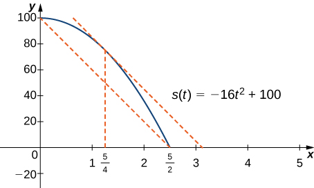
If a rock is dropped from a height of 100 ft, its position [latex]t[/latex] seconds after it is dropped until it hits the ground is given by the function [latex]s(t)=-16t^2+100[/latex].
- Determine how long it takes before the rock hits the ground.
- Find the average velocity [latex]v_{\text{avg}}[/latex] of the rock for when the rock is released and the rock hits the ground.
- Find the time [latex]t[/latex] guaranteed by the Mean Value Theorem when the instantaneous velocity of the rock is [latex]v_{\text{avg}}[/latex].
Suppose a ball is dropped from a height of 200 ft. Its position at time [latex]t[/latex] is [latex]s(t)=-16t^2+200[/latex]. Find the time [latex]t[/latex] when the instantaneous velocity of the ball equals its average velocity.
Hint
First, determine how long it takes for the ball to hit the ground. Then, find the average velocity of the ball from the time it is dropped until it hits the ground.
Corollaries of the Mean Value Theorem
Let’s now look at three corollaries of the Mean Value Theorem. These results have important consequences, which we use in upcoming sections.
At this point, we know the derivative of any constant function is zero. The Mean Value Theorem allows us to conclude that the converse is also true. In particular, if [latex]f^{\prime}(x)=0[/latex] for all [latex]x[/latex] in some interval [latex]I[/latex], then [latex]f(x)[/latex] is constant over that interval. This result may seem intuitively obvious, but it has important implications that are not obvious, and we discuss them shortly.
Corollary 1: Functions with a Derivative of Zero
Let [latex]f[/latex] be differentiable over an interval [latex]I[/latex]. If [latex]f^{\prime}(x)=0[/latex] for all [latex]x \in I[/latex], then [latex]f(x)[/latex] is constant for all [latex]x \in I[/latex].
Proof
Since [latex]f[/latex] is differentiable over [latex]I[/latex], [latex]f[/latex] must be continuous over [latex]I[/latex]. Suppose [latex]f(x)[/latex] is not constant for all [latex]x[/latex] in [latex]I[/latex]. Then there exist [latex]a,b \in I[/latex], where [latex]a \ne b[/latex] and [latex]f(a) \ne f(b)[/latex]. Choose the notation so that [latex]a Since [latex]f[/latex] is a differentiable function, by the Mean Value Theorem, there exists [latex]c \in (a,b)[/latex] such that Therefore, there exists [latex]c \in I[/latex] such that [latex]f^{\prime}(c) \ne 0[/latex], which contradicts the assumption that [latex]f^{\prime}(x)=0[/latex] for all [latex]x \in I[/latex]. □ From (Figure), it follows that if two functions have the same derivative, they differ by, at most, a constant. If [latex]f[/latex] and [latex]g[/latex] are differentiable over an interval [latex]I[/latex] and [latex]f^{\prime}(x)=g^{\prime}(x)[/latex] for all [latex]x \in I[/latex], then [latex]f(x)=g(x)+C[/latex] for some constant [latex]C[/latex].Corollary 2: Constant Difference Theorem
Proof
Let [latex]h(x)=f(x)-g(x)[/latex]. Then, [latex]h^{\prime}(x)=f^{\prime}(x)-g^{\prime}(x)=0[/latex] for all [latex]x \in I[/latex]. By Corollary 1, there is a constant [latex]C[/latex] such that [latex]h(x)=C[/latex] for all [latex]x \in I[/latex]. Therefore, [latex]f(x)=g(x)+C[/latex] for all [latex]x \in I[/latex].
□
The third corollary of the Mean Value Theorem discusses when a function is increasing and when it is decreasing. Recall that a function [latex]f[/latex] is increasing over [latex]I[/latex] if [latex]f(x_1)
This fact is important because it means that for a given function [latex]f[/latex], if there exists a function [latex]F[/latex] such that [latex]F^{\prime}(x)=f(x)[/latex]; then, the only other functions that have a derivative equal to [latex]f[/latex] are [latex]F(x)+C[/latex] for some constant [latex]C[/latex]. We discuss this result in more detail later in the chapter.
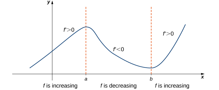
Figure 9. If a function has a positive derivative over some interval [latex]I[/latex], then the function increases over that interval [latex]I[/latex]; if the derivative is negative over some interval [latex]I[/latex], then the function decreases over that interval [latex]I[/latex].
Corollary 3: Increasing and Decreasing Functions
Let [latex]f[/latex] be continuous over the closed interval [latex][a,b][/latex] and differentiable over the open interval [latex](a,b)[/latex].
- If [latex]f^{\prime}(x)>0[/latex] for all [latex]x \in (a,b)[/latex], then [latex]f[/latex] is an increasing function over [latex][a,b][/latex].
- If [latex]f^{\prime}(x)<0[/latex] for all [latex]x \in (a,b)[/latex], then [latex]f[/latex] is a decreasing function over [latex][a,b][/latex].
Proof
We will prove 1.; the proof of 2. is similar. Suppose [latex]f[/latex] is not an increasing function on [latex]I[/latex]. Then there exist [latex]a[/latex] and [latex]b[/latex] in [latex]I[/latex] such that [latex]a Since [latex]f(a) \ge f(b)[/latex], we know that [latex]f(b)-f(a) \le 0[/latex]. Also, [latex]a However, [latex]f^{\prime}(x)>0[/latex] for all [latex]x \in I[/latex]. This is a contradiction, and therefore [latex]f[/latex] must be an increasing function over [latex]I[/latex]. □
Key Concepts
- If [latex]f[/latex] is continuous over [latex][a,b][/latex] and differentiable over [latex](a,b)[/latex] and [latex]f(a)=0=f(b)[/latex], then there exists a point [latex]c \in (a,b)[/latex] such that [latex]f^{\prime}(c)=0[/latex]. This is Rolle’s theorem.
- If [latex]f[/latex] is continuous over [latex][a,b][/latex] and differentiable over [latex](a,b)[/latex], then there exists a point [latex]c \in (a,b)[/latex] such that
[latex]f^{\prime}(c)=\frac{f(b)-f(a)}{b-a}[/latex].
This is the Mean Value Theorem.
- If [latex]f^{\prime}(x)=0[/latex] over an interval [latex]I[/latex], then [latex]f[/latex] is constant over [latex]I[/latex].
- If two differentiable functions [latex]f[/latex] and [latex]g[/latex] satisfy [latex]f^{\prime}(x)=g^{\prime}(x)[/latex] over [latex]I[/latex], then [latex]f(x)=g(x)+C[/latex] for some constant [latex]C[/latex].
- If [latex]f^{\prime}(x)>0[/latex] over an interval [latex]I[/latex], then [latex]f[/latex] is increasing over [latex]I[/latex]. If [latex]f^{\prime}(x)<0[/latex] over [latex]I[/latex], then [latex]f[/latex] is decreasing over [latex]I[/latex].
1. Why do you need continuity to apply the Mean Value Theorem? Construct a counterexample.
2. Why do you need differentiability to apply the Mean Value Theorem? Find a counterexample.
3. When are Rolle’s theorem and the Mean Value Theorem equivalent?
4. If you have a function with a discontinuity, is it still possible to have [latex]f^{\prime}(c)(b-a)=f(b)-f(a)[/latex]? Draw such an example or prove why not.
For the following exercises, determine over what intervals (if any) the Mean Value Theorem applies. Justify your answer.
5. [latex]y= \sin (\pi x)[/latex]
6. [latex]y=\frac{1}{x^3}[/latex]
7. [latex]y=\sqrt{4-x^2}[/latex]
8. [latex]y=\sqrt{x^2-4}[/latex]
9. [latex]y=\ln (3x-5)[/latex]
For the following exercises, graph the functions on a calculator and draw the secant line that connects the endpoints. Estimate the number of points [latex]c[/latex] such that [latex]f^{\prime}(c)(b-a)=f(b)-f(a)[/latex].
10. [T] [latex]y=3x^3+2x+1[/latex] over [latex][-1,1][/latex]
11. [T] [latex]y= \tan (\frac{\pi}{4}x)[/latex] over [latex][-\frac{3}{2},\frac{3}{2}][/latex]
12. [T] [latex]y=x^2 \cos (\pi x)[/latex] over [latex][-2,2][/latex]
13. [T] [latex]y=x^6-\frac{3}{4}x^5-\frac{9}{8}x^4+\frac{15}{16}x^3+\frac{3}{32}x^2+\frac{3}{16}x+\frac{1}{32}[/latex] over [latex][-1,1][/latex]
For the following exercises, use the Mean Value Theorem and find all points [latex]0 14. [latex]f(x)=x^3[/latex] 15. [latex]f(x)= \sin (\pi x)[/latex] 16. [latex]f(x)= \cos (2\pi x)[/latex] 17. [latex]f(x)=1+x+x^2[/latex] 18. [latex]f(x)=(x-1)^{10}[/latex] 19. [latex]f(x)=(x-1)^9[/latex] For the following exercises, show there is no [latex]c[/latex] such that [latex]f(1)-f(-1)=f^{\prime}(c)(2)[/latex]. Explain why the Mean Value Theorem does not apply over the interval [latex][-1,1][/latex] 20. [latex]f(x)=|x-\frac{1}{2}|[/latex] 21. [latex]f(x)=\frac{1}{x^2}[/latex] 22. [latex]f(x)=\sqrt{|x|}[/latex] 23. [latex]f(x)=⌊x⌋[/latex] (Hint: This is called the floor function and it is defined so that [latex]f(x)[/latex] is the largest integer less than or equal to [latex]x[/latex].) For the following exercises, determine whether the Mean Value Theorem applies for the functions over the given interval [latex][a,b][/latex]. Justify your answer. 24. [latex]y=e^x[/latex] over [latex][0,1][/latex] 25. [latex]y=\ln (2x+3)[/latex] over [latex][-\frac{3}{2},0][/latex] 26. [latex]f(x)= \tan (2\pi x)[/latex] over [latex][0,2][/latex] 27. [latex]y=\sqrt{9-x^2}[/latex] over [latex][-3,3][/latex] 28. [latex]y=\frac{1}{|x+1|}[/latex] over [latex][0,3][/latex] 29. [latex]y=x^3+2x+1[/latex] over [latex][0,6][/latex] 30. [latex]y=\frac{x^2+3x+2}{x}[/latex] over [latex][-1,1][/latex] 31. [latex]y=\frac{x}{ \sin (\pi x)+1}[/latex] over [latex][0,1][/latex] 32. [latex]y=\ln (x+1)[/latex] over [latex][0,e-1][/latex] 33. [latex]y=x \sin (\pi x)[/latex] over [latex][0,2][/latex] 34. [latex]y=5+|x|[/latex] over [latex][-1,1][/latex] For the following exercises, consider the roots of the equation. 35. Show that the equation [latex]y=x^3+3x^2+16[/latex] has exactly one real root. What is it? 36. Find the conditions for exactly one root (double root) for the equation [latex]y=x^2+bx+c[/latex] 37. Find the conditions for [latex]y=e^x-b[/latex] to have one root. Is it possible to have more than one root? For the following exercises, use a calculator to graph the function over the interval [latex][a,b][/latex] and graph the secant line from [latex]a[/latex] to [latex]b[/latex]. Use the calculator to estimate all values of [latex]c[/latex] as guaranteed by the Mean Value Theorem. Then, find the exact value of [latex]c[/latex], if possible, or write the final equation and use a calculator to estimate to four digits. 38. [T] [latex]y= \tan (\pi x)[/latex] over [latex][-\frac{1}{4},\frac{1}{4}][/latex] 39. [T] [latex]y=\frac{1}{\sqrt{x+1}}[/latex] over [latex][0,3][/latex] 40. [T] [latex]y=|x^2+2x-4|[/latex] over [latex][-4,0][/latex] 41. [T] [latex]y=x+\frac{1}{x}[/latex] over [latex][\frac{1}{2},4][/latex] 42. [T] [latex]y=\sqrt{x+1}+\frac{1}{x^2}[/latex] over [latex][3,8][/latex] 43. At 10:17 a.m., you pass a police car at 55 mph that is stopped on the freeway. You pass a second police car at 55 mph at 10:53 a.m., which is located 39 mi from the first police car. If the speed limit is 60 mph, can the police cite you for speeding? 44. Two cars drive from one spotlight to the next, leaving at the same time and arriving at the same time. Is there ever a time when they are going the same speed? Prove or disprove. 45. Show that [latex]y= \sec^2 x[/latex] and [latex]y= \tan^2 x[/latex] have the same derivative. What can you say about [latex]y= \sec^2 x - \tan^2 x[/latex]? 46. Show that [latex]y= \csc^2 x[/latex] and [latex]y= \cot^2 x[/latex] have the same derivative. What can you say about [latex]y= \csc^2 x - \cot^2 x[/latex]?
Glossary
- mean value theorem
- if [latex]f[/latex] is continuous over [latex][a,b][/latex] and differentiable over [latex](a,b)[/latex], then there exists [latex]c \in (a,b)[/latex] such that
[latex]f^{\prime}(c)=\frac{f(b)-f(a)}{b-a}[/latex]
- rolle’s theorem
- if [latex]f[/latex] is continuous over [latex][a,b][/latex] and differentiable over [latex](a,b)[/latex], and if [latex]f(a)=f(b)[/latex], then there exists [latex]c \in (a,b)[/latex] such that [latex]f^{\prime}(c)=0[/latex]
Candela Citations
- Calculus I. Provided by: OpenStax. Located at: http://cnx.org/contents/8b89d172-2927-466f-8661-01abc7ccdba4@2.89. License: CC BY-NC-SA: Attribution-NonCommercial-ShareAlike. License Terms: Download for free at http://cnx.org/contents/8b89d172-2927-466f-8661-01abc7ccdba4@2.89

Hint
Find all values [latex]c[/latex], where [latex]f^{\prime}(c)=0[/latex].