Probability Distribution

Matter and photons are waves, implying they are spread out over some distance. What is the position of a particle, such as an electron? Is it at the center of the wave? The answer lies in how you measure the position of an electron. Experiments show that you will find the electron at some definite location, unlike a wave. But if you set up exactly the same situation and measure it again, you will find the electron in a different location, often far outside any experimental uncertainty in your measurement. Repeated measurements will display a statistical distribution of locations that appears wavelike. (See Figure 1.)

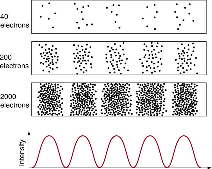
Figure 1. The building up of the diffraction pattern of electrons scattered from a crystal surface. Each electron arrives at a definite location, which cannot be precisely predicted. The overall distribution shown at the bottom can be predicted as the diffraction of waves having the de Broglie wavelength of the electrons.

After de Broglie proposed the wave nature of matter, many physicists, including Schrödinger and Heisenberg, explored the consequences. The idea quickly emerged that, because of its wave character, a particle’s trajectory and destination cannot be precisely predicted for each particle individually. However, each particle goes to a definite place (as illustrated in Figure 1). After compiling enough data, you get a distribution related to the particle’s wavelength and diffraction pattern. There is a certain probability of finding the particle at a given location, and the overall pattern is called a probability distribution. Those who developed quantum mechanics devised equations that predicted the probability distribution in various circumstances.

It is somewhat disquieting to think that you cannot predict exactly where an individual particle will go, or even follow it to its destination. Let us explore what happens if we try to follow a particle. Consider the double-slit patterns obtained for electrons and photons in Figure 2. First, we note that these patterns are identical, following d sin θ = mλ, the equation for double-slit constructive interference developed in Photon Energies and the Electromagnetic Spectrum, where d is the slit separation and λ is the electron or photon wavelength.

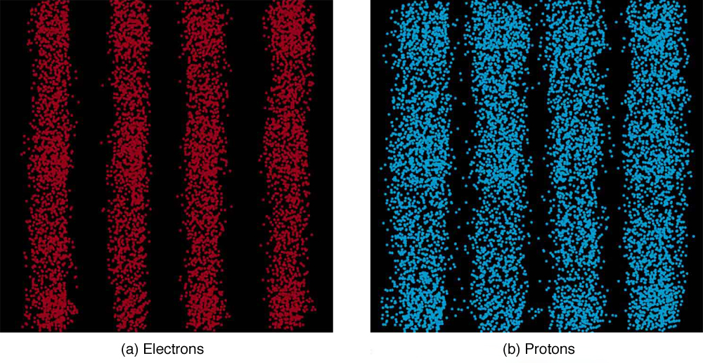
Figure 2. Double-slit interference for electrons (a) and photons (b) is identical for equal wavelengths and equal slit separations. Both patterns are probability distributions in the sense that they are built up by individual particles traversing the apparatus, the paths of which are not individually predictable.

Both patterns build up statistically as individual particles fall on the detector. This can be observed for photons or electrons—for now, let us concentrate on electrons. You might imagine that the electrons are interfering with one another as any waves do. To test this, you can lower the intensity until there is never more than one electron between the slits and the screen. The same interference pattern builds up! This implies that a particle’s probability distribution spans both slits, and the particles actually interfere with themselves. Does this also mean that the electron goes through both slits? An electron is a basic unit of matter that is not divisible. But it is a fair question, and so we should look to see if the electron traverses one slit or the other, or both. One possibility is to have coils around the slits that detect charges moving through them. What is observed is that an electron always goes through one slit or the other; it does not split to go through both. But there is a catch. If you determine that the electron went through one of the slits, you no longer get a double slit pattern—instead, you get single slit interference. There is no escape by using another method of determining which slit the electron went through. Knowing the particle went through one slit forces a single-slit pattern. If you do not observe which slit the electron goes through, you obtain a double-slit pattern.

Heisenberg Uncertainty

How does knowing which slit the electron passed through change the pattern? The answer is fundamentally important—measurement affects the system being observed. Information can be lost, and in some cases it is impossible to measure two physical quantities simultaneously to exact precision. For example, you can measure the position of a moving electron by scattering light or other electrons from it. Those probes have momentum themselves, and by scattering from the electron, they change its momentum in a manner that loses information. There is a limit to absolute knowledge, even in principle.

Figure 3. Werner Heisenberg was one of the best of those physicists who developed early quantum mechanics. Not only did his work enable a description of nature on the very small scale, it also changed our view of the availability of knowledge. Although he is universally recognized for his brilliance and the importance of his work (he received the Nobel Prize in 1932, for example), Heisenberg remained in Germany during World War II and headed the German effort to build a nuclear bomb, permanently alienating himself from most of the scientific community. (credit: Author Unknown, via Wikimedia Commons)

It was Werner Heisenberg who first stated this limit to knowledge in 1929 as a result of his work on quantum mechanics and the wave characteristics of all particles. (See Figure 3). Specifically, consider simultaneously measuring the position and momentum of an electron (it could be any particle). There is an uncertainty in position Δx that is approximately equal to the wavelength of the particle. That is, Δx ≈ λ.

As discussed above, a wave is not located at one point in space. If the electron’s position is measured repeatedly, a spread in locations will be observed, implying an uncertainty in position Δx. To detect the position of the particle, we must interact with it, such as having it collide with a detector. In the collision, the particle will lose momentum. This change in momentum could be anywhere from close to zero to the total momentum of the particle, [latex]p=\frac{h}{\lambda}\\[/latex]. It is not possible to tell how much momentum will be transferred to a detector, and so there is an uncertainty in momentum Δp, too. In fact, the uncertainty in momentum may be as large as the momentum itself, which in equation form means that [latex]\Delta{p}\approx\frac{h}{\lambda}\\[/latex].

The uncertainty in position can be reduced by using a shorter-wavelength electron, since Δx ≈ λ. But shortening the wavelength increases the uncertainty in momentum, since [latex]p=\frac{h}{\lambda}\\[/latex]. Conversely, the uncertainty in momentum can be reduced by using a longer-wavelength electron, but this increases the uncertainty in position. Mathematically, you can express this trade-off by multiplying the uncertainties. The wavelength cancels, leaving ΔxΔp ≈ h.

So if one uncertainty is reduced, the other must increase so that their product is ≈h.

With the use of advanced mathematics, Heisenberg showed that the best that can be done in a simultaneous measurement of position and momentum is [latex]\Delta{x}\Delta{p}\ge\frac{h}{4\pi}\\[/latex].

This is known as the Heisenberg uncertainty principle. It is impossible to measure position x and momentum p simultaneously with uncertainties Δx and Δp that multiply to be less than [latex]\frac{h}{4\pi}\\[/latex]. Neither uncertainty can be zero. Neither uncertainty can become small without the other becoming large. A small wavelength allows accurate position measurement, but it increases the momentum of the probe to the point that it further disturbs the momentum of a system being measured. For example, if an electron is scattered from an atom and has a wavelength small enough to detect the position of electrons in the atom, its momentum can knock the electrons from their orbits in a manner that loses information about their original motion. It is therefore impossible to follow an electron in its orbit around an atom. If you measure the electron’s position, you will find it in a definite location, but the atom will be disrupted. Repeated measurements on identical atoms will produce interesting probability distributions for electrons around the atom, but they will not produce motion information. The probability distributions are referred to as electron clouds or orbitals. The shapes of these orbitals are often shown in general chemistry texts and are discussed in The Wave Nature of Matter Causes Quantization.

Why don’t we notice Heisenberg’s uncertainty principle in everyday life? The answer is that Planck’s constant is very small. Thus the lower limit in the uncertainty of measuring the position and momentum of large objects is negligible. We can detect sunlight reflected from Jupiter and follow the planet in its orbit around the Sun. The reflected sunlight alters the momentum of Jupiter and creates an uncertainty in its momentum, but this is totally negligible compared with Jupiter’s huge momentum. The correspondence principle tells us that the predictions of quantum mechanics become indistinguishable from classical physics for large objects, which is the case here.

Heisenberg Uncertainty for Energy and Time

There is another form of Heisenberg’s uncertainty principle for simultaneous measurements of energy and time. In equation form, [latex]\Delta{E}\Delta{t}\ge\frac{h}{4\pi}\\[/latex], where ΔE is the uncertainty in energy and Δt is the uncertainty in time. This means that within a time interval Δt, it is not possible to measure energy precisely—there will be an uncertainty ΔE in the measurement. In order to measure energy more precisely (to make ΔE smaller), we must increase Δt. This time interval may be the amount of time we take to make the measurement, or it could be the amount of time a particular state exists, as in the next Example 2.

The uncertainty principle for energy and time can be of great significance if the lifetime of a system is very short. Then Δt is very small, and ΔE is consequently very large. Some nuclei and exotic particles have extremely short lifetimes (as small as 10⁻²⁵ s), causing uncertainties in energy as great as many GeV (10⁹ eV). Stored energy appears as increased rest mass, and so this means that there is significant uncertainty in the rest mass of short-lived particles. When measured repeatedly, a spread of masses or decay energies are obtained. The spread is ΔE. You might ask whether this uncertainty in energy could be avoided by not measuring the lifetime. The answer is no. Nature knows the lifetime, and so its brevity affects the energy of the particle. This is so well established experimentally that the uncertainty in decay energy is used to calculate the lifetime of short-lived states. Some nuclei and particles are so short-lived that it is difficult to measure their lifetime. But if their decay energy can be measured, its spread is ΔE, and this is used in the uncertainty principle [latex]\left(\Delta{E}\Delta{t}\ge\frac{h}{4\pi}\right)\\[/latex] to calculate the lifetime Δt.

There is another consequence of the uncertainty principle for energy and time. If energy is uncertain by ΔE, then conservation of energy can be violated by ΔE for a time Δt. Neither the physicist nor nature can tell that conservation of energy has been violated, if the violation is temporary and smaller than the uncertainty in energy. While this sounds innocuous enough, we shall see in later chapters that it allows the temporary creation of matter from nothing and has implications for how nature transmits forces over very small distances.

Finally, note that in the discussion of particles and waves, we have stated that individual measurements produce precise or particle-like results. A definite position is determined each time we observe an electron, for example. But repeated measurements produce a spread in values consistent with wave characteristics. The great theoretical physicist Richard Feynman (1918–1988) commented, “What there are, are particles.” When you observe enough of them, they distribute themselves as you would expect for a wave phenomenon. However, what there are as they travel we cannot tell because, when we do try to measure, we affect the traveling.

Section Summary

• Matter is found to have the same interference characteristics as any other wave.
• There is now a probability distribution for the location of a particle rather than a definite position.
• Another consequence of the wave character of all particles is the Heisenberg uncertainty principle, which limits the precision with which certain physical quantities can be known simultaneously. For position and momentum, the uncertainty principle is [latex]\Delta{x}\Delta{p}\ge\frac{h}{4\pi}\\[/latex], where Δx is the uncertainty in position and Δp is the uncertainty in momentum.
• For energy and time, the uncertainty principle is [latex]\Delta{E}\Delta{t}\ge\frac{h}{4\pi}\\[/latex] whereΔE is the uncertainty in energy andΔt is the uncertainty in time.
• These small limits are fundamentally important on the quantum-mechanical scale.

Glossary

Heisenberg’s uncertainty principle: a fundamental limit to the precision with which pairs of quantities (momentum and position, and energy and time) can be measured

uncertainty in energy: lack of precision or lack of knowledge of precise results in measurements of energy

uncertainty in time: lack of precision or lack of knowledge of precise results in measurements of time

uncertainty in momentum: lack of precision or lack of knowledge of precise results in measurements of momentum

uncertainty in position: lack of precision or lack of knowledge of precise results in measurements of position

probability distribution: the overall spatial distribution of probabilities to find a particle at a given location