Learning Objectives
- Describe the sampling distribution of sample means.
Our next goal is to determine how the size of the sample affects the variability we see in sample means.
Example
Sample Size Affects Variability of Sample Means
We assumed that the population of individual babies has a mean of µ = 3,500 grams and a standard deviation of σ = 500 grams. We selected a random sample of babies to test our assumptions about the population.
We saw previously that for this population of babies, it was not surprising to see a random sample of 9 babies with a mean birth weight of 3,400 grams. So a sample with a mean of 3,400 does not suggest that the town’s mean birth weight is less than 3,500 grams this year.
What if we increase the sample size? Will our conclusion change? That is, if the mean birth weight of 3,400 grams comes from a larger sample of babies, does the sample provide stronger evidence that the town’s mean birth weight is less than 3,500 grams?
To investigate this question, we ran the simulation for different sample sizes. For each sample size, we collected 1,000 random samples and recorded the sample means.
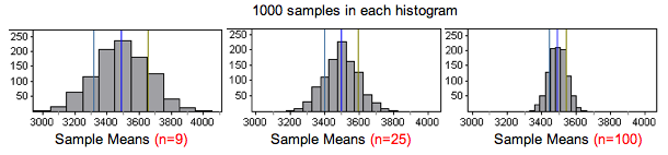
When we compare the histograms of sample means, we notice the following:
- Center: The center is not affected by sample size. The mean of the sample means is always approximately the same as the population mean µ = 3,500.
- Spread: The spread is smaller for larger samples, so the standard deviation of the sample means decreases as sample size increases. This is not surprising because we observed a similar trend with sample proportions.
- Shape: The sampling distributions all appear approximately normal. This is not surprising because the distribution of birth weights in the population has a normal shape.
Based on the histograms, it appears that sample size will change our conclusion about the population’s mean birth weight this year. Suppose our sample mean of 3,400 grams came from a random sample of 100 babies. Means from samples this large did not vary much. We marked this sample result in a histogram for samples of size 100.
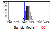
For n = 100, a sample mean of 3,400 grams is an unlikely result. It gives fairly strong evidence that the population’s mean birth weight is less than 3,500 grams.
From advanced probability theory, we have a probability model for the sampling distribution of sample means. The model reinforces what we have already observed about the center and gives more precise information about the relationship between sample size and spread.
The Theoretical Probability Model for the Sampling Distribution of Sample Means
Suppose a population has a mean µ and a standard deviation of σ. The distribution of all possible sample means from this population will have a mean of µ and a standard deviation of [latex]σ\text{}/\sqrt{n}[/latex].
Learn By Doing
Learn By Doing
Let’s compare and contrast what we know about the sampling distributions for sample means and sample proportions.
| Sampling Distribution | |||||
|---|---|---|---|---|---|
| Variable | Parameter | Statistic | Center | Spread | Shape |
| Categorical (example: left-handed or not) | p = population proportion | [latex]\stackrel{ˆ}{p}[/latex] = sample proportion | p | [latex]\sqrt{\frac{p(1-p)}{n}}[/latex] | Normal when np ≥ 10 and n(1 – p) ≥ 10 |
| Quantitative (example: age) | μ = population mean, σ = population standard deviation | [latex]\overline{x}[/latex] = sample mean | μ | [latex]\frac{\sigma }{\sqrt{n}}[/latex] | When will the distribution of sample means be approximately normal? |
We investigate the conditions that guarantee a normal sampling distribution for sample means on the next page.
Candela Citations
- Concepts in Statistics. Provided by: Open Learning Initiative. Located at: http://oli.cmu.edu. License: CC BY: Attribution