Learning Objectives
- Conduct a chi-square goodness-of-fit test. Interpret the conclusion in context.
Here we continue with the details of the chi-square goodness-of-fit hypothesis test. A goodness-of-fit test determines whether or not the distribution of a categorical variable in a sample fits a claimed distribution in the population. The chi-square test statistic is our measure of how much the sample distribution deviates from the population distribution.
As with other hypothesis tests, we need to be able to model the variability we expect in samples if the null hypothesis is true. Then we can determine whether the chi-square test statistic from the data is unusual or typical. An unusual χ2 value suggests that there are statistically significant differences between the sample data and the null distribution and provides evidence against the null hypothesis. This is the same logic we have been applying with hypothesis testing.
Example
Distribution of Color in Plain M&M Candies
Recall the claim made by the manufacturer of M&M candy: the color distribution for plain chocolate M&Ms is 13% brown, 13% red, 14% yellow, 24% blue, 20% orange, 16% green. We used this distribution as our null hypothesis.
- H0: The color distribution for plain M&Ms is 13% brown, 13% red, 14% yellow, 24% blue, 20% orange, 16% green.
- Ha: The color distribution for plain M&Ms is different from the distribution stated in the null hypothesis.
Suppose we buy a large bag of plain M&M candies to test these hypotheses. We randomly select 300 from the bag and view this as a random sample from the population of all plain M&M candies. Our observed counts along with the expected counts are shown in the following ribbon chart and the table. Recall that the expected counts come from the null hypothesis.

We see that the sample distribution is very close to the null distribution for some colors and not others. The deviation appears largest for blue and orange. When we calculate the chi-square statistic, we see that these colors contribute the most to the chi-square value.
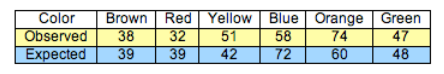
[latex]\begin{array}{l}\text{}\text{}\text{}\text{}\text{}\text{}\text{}\text{}\text{}\text{}\text{}\text{}\text{}\mathrm{brown}\text{}\text{}\text{}\text{}\text{}\text{}\text{}\text{}\text{}\text{}\text{}\text{}\text{}\text{}\text{}\mathrm{red}\text{}\text{}\text{}\text{}\text{}\text{}\text{}\text{}\text{}\text{}\text{}\text{}\text{}\text{}\text{}\text{}\mathrm{yellow}\text{}\text{}\text{}\text{}\text{}\text{}\text{}\text{}\text{}\text{}\text{}\text{}\text{}\mathrm{blue}\text{}\text{}\text{}\text{}\text{}\text{}\text{}\text{}\text{}\text{}\text{}\text{}\text{}\text{}\text{}\mathrm{orange}\text{}\text{}\text{}\text{}\text{}\text{}\text{}\text{}\text{}\text{}\text{}\text{}\text{}\mathrm{green}\\ {\mathrm{χ}}^{2}=\frac{{(38-39)}^{2}}{39}+\frac{{(32-39)}^{2}}{39}+\frac{{(51-42)}^{2}}{42}+\frac{{(58-72)}^{2}}{72}+\frac{{(74-60)}^{2}}{60}+\frac{{(47-48)}^{2}}{48}\\ \text{}\text{}\text{}\text{}\\ \text{}\text{}\text{}\text{}\text{}\approx \text{}\text{}\text{}\text{}0.03\text{}\text{}\text{}\text{}\text{}\text{}+\text{}\text{}\text{}\text{}\text{}\text{}\text{}\text{}1.26\text{}\text{}\text{}\text{}\text{}+\text{}\text{}\text{}\text{}\text{}1.93\text{}\text{}\text{}\text{}\text{}+\text{}\text{}\text{}\text{}\text{}2.72\text{}\text{}\text{}\text{}\text{}\text{}+\text{}\text{}\text{}\text{}\text{}\text{}3.27\text{}\text{}\text{}\text{}\text{}\text{}+\text{}\text{}\text{}\text{}\text{}\text{}\text{}0.02=9.23\text{}\end{array}[/latex]
What can we conclude? Is this chi-square value unusual or typical? To answer these questions, we must take many random samples from the population described by the null hypothesis. As we have done before, we use a simulation to take random samples. We do this in the next activity.
Learn By Doing
Reasoning from the Chi-Square Sampling Distribution
Click here to open the simulation.
Learn By Doing
Reasoning from the Chi-Square Sampling Distribution
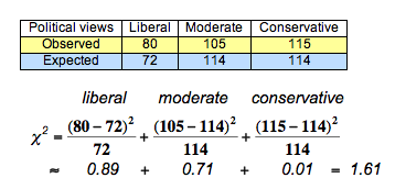
Recall the distribution of political views for registered voters in 2008: 24% liberal, 38% moderate, and 38% conservative. We want to determine if the distribution is the same this year.
- H0: The distribution of political views this year is 0.24 liberal, 0.38 moderate, 0.38 conservative.
- Ha: The distribution of political views this year differs from the 2008 distribution stated in the null hypothesis.
Previously, we used the data shown in the table to calculate the chi-square test statistic of 1.61.
What can we conclude?
Click here to open the simulation. Use this simulation to select at least 40 random samples from the null distribution.
Use the simulation below these next questions to select at least 40 random samples from the null distribution.
Now mark each conclusion valid or invalid.
In the previous activities, we based our conclusions on a relatively small number of random samples. If we continued taking random samples, the resulting distribution of chi-square statistics has a pattern that can be described by a mathematical model, called the chi-square distribution. As with other models for sampling distributions, this model is a probability model. The total area under the curve equals 1. We again use the area under the curve to represent the probability of sample results occurring if the null hypothesis is true. This means we again use the mathematical model with technology to find a P-value.
The Chi-Square Distribution
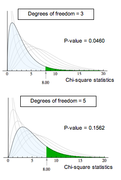
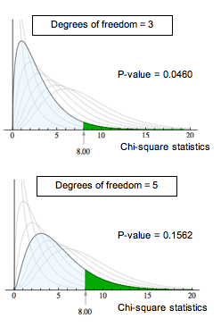
Unlike other sampling distributions we have studied, the chi-square model does not have a normal shape. It is skewed to the right. Like the T-model, the chi-square model is a family of curves that depend on degrees of freedom. For a chi-square goodness-of-fit test, the degrees of freedom is the number categories minus 1. (Sometimes this is written (r − 1), where r represents “rows” in the one-way table of observed counts.) The mean of the chi-square distribution is equal to the degrees of freedom.
A chi-square model is a good fit for the distribution of the chi-square test statistic only if the following conditions are met:
- The sample is randomly selected.
- All of the expected counts are 5 or greater.
If these conditions are met, we use the chi-square distribution to find the P-value. We use the same logic that we use in all hypothesis tests to draw a conclusion based on the P-value. If the P-value is at least as small as the significance level, we reject the null hypothesis and accept the alternative hypothesis.
The P-value is the likelihood that results from random samples have a χ2 value equal to or greater than that calculated from the data. As before, the P-value is a conditional probability based on the condition that the null hypothesis is true. For different degrees of freedom, the same χ2 value gives different P-values. For example, a chi-square value of 8 is statistically significant for α = 0.05 with 3 degrees of freedom. This is not true for 5 degrees of freedom. As shown below, this is due to the change in the chi-square curve.
Learn By Doing
Hypothesis Test about the Color Distribution for Plain M&Ms
Recall the hypothesis test about the color distribution for plain M&Ms.
- H0: The color distribution for plain M&Ms is 13% brown, 13% red, 14% yellow, 24% blue, 20% orange, 16% green.
- Ha: The color distribution for plain M&Ms is different from the distribution stated in the null hypothesis.
From the null hypothesis, we determined the expected counts for a sample of 300. A random sample of 300 M&Ms gave the observed counts shown in the table. We calculated a chi-square statistic of 9.23.

Click here to open the simulation.
Comment
Goodness-of-fit is an extension of the hypothesis test for one population proportion that we learned in Inference for One Proportion. Both of these hypothesis tests focus on a categorical variable in one population. In the hypothesis test for one population proportion, we focus on one category of the variable that we call “a success.” We make a claim about the proportion of “successes” in the population. For example, we previously investigated the claim that 20% of plain M&Ms are orange. In a chi-square goodness-of-fit test, we focus on the entire distribution of categories for the variable. So we investigate a claim that the color distribution for plain M&Ms is 13% brown, 13% red, 14% yellow, 24% blue, 20% orange, 16% green. The chi-square goodness-of-fit test does not give information about the deviation for specific categories. It gives a more general conclusion of “seems to fit the null distribution” or “does not fit the null distribution.”
Let’s Summarize
In “Chi-Square Test for One-Way Tables,” we learned an inference procedure called the chi-square goodness-of-fit test. A goodness-of-fit test determines if the distribution of a categorical variable in a sample fits a claimed distribution in the population, or not.
We can answer the following research questions with a chi-square goodness-of-fit test:
- The distribution of blood types in the United States is 45% type O, 41% type A, 10% type B, and 4% type AB. Is the distribution of blood types the same in China?
- The Mars Company claims that 24% of M&M plain milk chocolate candies are blue, 13% brown, 16% green, 20% orange, 10% red, and 14% yellow. Do the M&Ms in our sample suggest that the color distribution is different?
The Chi-Square Test Statistic and Distribution
The chi-square test statistic χ2 measures how far the observed data are from the null hypothesis by comparing observed counts and expected counts. Expected counts are the counts we expect to see if the null hypothesis is true.
[latex]{\chi }^{2}\text{}=\text{}∑\frac{{(\mathrm{observed}-\mathrm{expected})}^{2}}{\mathrm{expected}}[/latex]
The chi-square model is a family of curves that depend on degrees of freedom. For a one-way table the degrees of freedom equals (r – 1). All chi-square curves are skewed to the right with a mean equal to the degrees of freedom.
A chi-square model is a good fit for the distribution of the chi-square test statistic only if the following conditions are met:
- The sample is randomly selected.
- All expected counts are 5 or greater.
If these conditions are met, we use the chi-square distribution to find the P-value. We use the same logic that we use in all hypothesis tests to draw a conclusion based on the P-value. If the P-value is at least as small as the significance level, we reject the null hypothesis and accept the alternative hypothesis. The P-value is the likelihood that results from random samples have a χ2 value equal to or greater than that calculated from the data if the null hypothesis is true. For different degrees of freedom, the same χ2 value gives different P-values.
Candela Citations
- Concepts in Statistics. Provided by: Open Learning Initiative. Located at: http://oli.cmu.edu. License: CC BY: Attribution