Learning Objectives
- Explain that the inverse of a linear function is a function
- Graph the inverse of a linear function
- Find the inverse function of a linear function algebraically
The Inverse of a Function
We learned in section 1.3 that the inverse of a function may be obtained by exchanging the domain and range (or the input and output) of the function. For example, the inverse of the function [latex]\{(1, 2), (3, 4), (5, 6)\}[/latex] is [latex]\{(2, 1), (4, 3), (6, 5)\}[/latex]. All we have to do is switch the [latex]x[/latex]– and [latex]y[/latex]-values in the ordered pairs. Note that the inverse of a function may or may not be a function. Figure 1 shows a function and its inverse where the inverse is a function. Figure 2 shows a function and its inverse where the inverse is NOT a function. A function will have an inverse function only if the original function is one-to-one. If the inverse of a function [latex]f[/latex] is also a function, we may use the notation [latex]f^{-1}[/latex] to name the inverse function. It is important to note that the “–1” is not an exponent. It is a superscript meaning “inverse”. The notation [latex]f^{-1}[/latex] means the inverse function of the function [latex]f[/latex]. This function [latex]f^{-1}[/latex] is a completely different function from [latex]f[/latex].
|
True 1 – 1 function and its inverse
|
Not a 1 – 1 function
|
|---|---|

Figure 1. The inverse of a 1-1 function is a 1-1 function. |

Figure 2. A function that is not 1-1 has an inverse that is not a function. |
The Inverse of a Linear Function
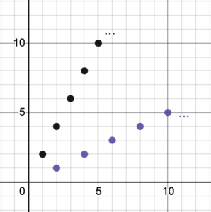
A linear function [latex]f(x)=mx+b[/latex] with [latex]m\ne0[/latex] is a one-to-one mapping of [latex]x[/latex] to the function value [latex]f(x)[/latex] because each point on the graph of the function has a unique input and a unique output. There are no two points that have the same input ([latex]x[/latex]-coordinate) or the same output ([latex]y[/latex]-coordinate). Figure 3 illustrates some points (or solution pairs) on the graph of the function [latex]f(x)=2x[/latex] as well as the corresponding points on the graph of the inverse function [latex]f^{-1}(x)[/latex], which are found by simply switching the [latex]x[/latex]– and [latex]y[/latex]-coordinates of the original points. Both sets of points show a one-to-one mapping. This is an example of the fact that the inverse of a linear function with a non-zero slope is also a one-to-one linear function.

Figure 3. Points (solution pairs) on the graph of the function [latex]f(x) = 2x[/latex] and its inverse.
A linear function with a zero slope (a horizontal line), i.e., [latex]f(x)=b[/latex], has an inverse that is not a function, [latex]x=b[/latex] (a vertical line). A horizontal line does not represent a one-to-one function, which is why its inverse is not a function (figure 4).

Figure 4. Horizontal line is a function; vertical line is not a function.
Graphing the Inverse of a Linear Function
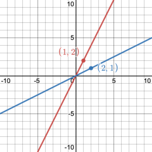
To graph the inverse of a linear function, we may start by finding two or more points (solution pairs) on the graph of the linear function. Then we simply switch the [latex]x[/latex]– and [latex]y[/latex]-coordinates of each point to find points that lie on the graph of the inverse function. We can then use these points to graph the inverse function. For example, (0, 0) and (1, 2) are two points that lie on the graph of the function [latex]f(x)=2x[/latex]. To graph the inverse function, we switch the [latex]x[/latex]– and [latex]y[/latex]-coordinates of these points to get (0, 0) and (2, 1). Therefore, the graph of the inverse function will be the line that passes through the two points (0, 0) and (2, 1) (See Figure 5).

Figure 5. Graph of the function [latex]f(x)=2x[/latex] and its inverse.
Example 1
Use the graphs of the linear functions to graph their inverse function.
| Problem 1 | Problem 2 |
|---|---|

[latex]f(x)=4x-2[/latex] |

[latex]f(x)=-\frac{2}{3}x+5[/latex] |
Solution
| Problem 1 |
Problem 2 |
|---|---|
|
Choose 2 (or more) points on the original line: (0, –2) and (1, 2) Reverse the [latex]x[/latex]– and [latex]y[/latex]-coordinates: (–2, 0) and (2, 1) Plot the new points. The line that passes through them is the inverse function. 
[latex]f(x)=4x-2[/latex] and its inverse
|
Choose 2 (or more) points on the original line: (0, 5) and (6, 1) Reverse the [latex]x[/latex]– and [latex]y[/latex]-coordinates: (5, 0) and (1, 6) Plot the new points. The line that passes through them is the inverse function. 
[latex]f(x)=-\frac{2}{3}x+5[/latex] and its inverse |
Try It 1
Use the graphs of the linear functions to graph their inverse function.
| Problem 1 | Problem 2 |

[latex]f(x)=-3x+5[/latex] |

[latex]f(x)=\frac{4}{3}x+2[/latex] |
Example 2
Graph the function [latex]f(x)=\frac{2}{5}x+2[/latex], then graph its inverse.
Solution
To graph [latex]f(x)=\frac{2}{5}x+2[/latex] we can either use a table of values or use the slope and [latex]y[/latex]-intercept.
The slope of the line is [latex]m=\frac{2}{5}[/latex] and the [latex]y[/latex]-intercept is (0, 2).
To graph the line, we start at (0, 2) then run 5 units to the right and 2 units up to get to (5, 4).

[latex]f(x)=\frac{2}{5}x+2[/latex]
Now reverse the points (0, 2) and (5, 4) to (2, 0) and (4, 5) and draw the line of the inverse function through these new points.

[latex]f(x)=\frac{2}{5}x+2[/latex] and its inverse
Try It 2
Graph the function [latex]f(x)=\frac{1}{3}x-4[/latex], then graph its inverse.
Inverse Functions and Symmetry
As we saw in chapter 1, the graph of any function and its inverse are symmetric across the line [latex]y=x[/latex]. For example, figure 6 shows the graph of [latex]f(x)=\frac{2}{5}x+2[/latex] and its inverse. With the added line [latex]y=x[/latex], we can see that the two lines are symmetric (mirror images of one another) across the line [latex]y=x[/latex].

Figure 6. [latex]f(x)=\frac{2}{5}x+2[/latex] and its inverse
Notice the [latex]x[/latex]– and [latex]y[/latex]-intercepts. The [latex]y[/latex]-intercept of (0, 2) in the original function (blue line) reflects to the [latex]x[/latex]-intercept (2, 0) in the inverse function (green line). Also, the [latex]x[/latex]-intercept of (–5, 0) in the original function (blue line) reflects to the [latex]y[/latex]-intercept (0, –5) in the inverse function (green line).
The slopes of each function are also related. The function [latex]f(x)[/latex] has a slope of [latex]\frac{2}{5}[/latex], while the inverse function [latex]f^{-1}(x)[/latex] has a slope of [latex]\frac{5}{2}[/latex]. The slopes of inverse functions are reciprocals of each other. This is because the slope of a function is [latex]\dfrac{\text{change in y}}{\text{change in x}}[/latex]. The slope of the inverse function becomes [latex]\dfrac{\text{change in x}}{\text{change in y}}[/latex].
Since we know the slopes are reciprocals and the [latex]y[/latex]-intercept of the inverse function is the flipped coordinates of the [latex]x[/latex]-intercept of the original function, we can find the equation of the inverse function: [latex]m=\frac{5}{2},\;b=-5[/latex] so [latex]f^{-1}(x)=\frac{5}{2}x-5[/latex].
Example 3
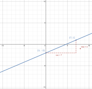
Graph the function [latex]g(x)=\frac{3}{7}x-2[/latex] then use symmetry to graph its inverse. Write the equation of the inverse function.
Solution
To graph [latex]g(x)=\frac{3}{7}x-2[/latex], we can start at the [latex]y[/latex]-intercept (0, –2) then use the slope of [latex]\frac{3}{7}[/latex] to run 7 and rise 3 to get to another point on the line: (7, 1). Then draw the line through these points.

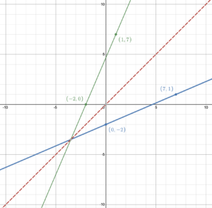
To graph the inverse function, we can draw the line [latex]y=x[/latex] then reflect points on the line of the original function across [latex]y=x[/latex] to get points on the inverse function. Then we can draw the line of the inverse function.

To write the equation of the inverse function, we know that the slope is [latex]\frac{7}{3}[/latex]; the reciprocal of the slope of the original function.
From the graph, the [latex]y[/latex]-intercept is fractional but we know that the inverse goes through the point (–2, 0); the flipped point of (0 –2) on the original function.
The inverse function is linear, so has the form [latex]f(x)=mx+b=\frac{7}{3}x+b[/latex] with the substituted slope.
To find [latex]b[/latex], we can use the point (–2, 0):
[latex]\begin{aligned}f(x)&=\frac{7}{3}x+b\\ 0&=\frac{7}{3}\cdot (-2)+b\\ 0&=\frac{-14}{3}+b\\b&= \frac{14}{3}\end{aligned}[/latex]
Consequently the inverse function is [latex]g^{-1}(x)=\frac{7}{3}x+\frac{14}{3}[/latex].
Try It 3
Graph the function [latex]g(x)=\frac{1}{2}x+3[/latex] then use symmetry to graph its inverse. Write the equation of the inverse function.
Figure 7 demonstrates the symmetry across the line [latex]y=x[/latex] of a function and its inverse. Each point on the line of the original function has a reflected point across [latex]y=x[/latex].
Figure 7. The symmetry of a function and its inverse.
The Algebraic Inverse Function of a Linear Function
We have learned that to graph an inverse function, we simply switch the [latex]x[/latex]– and [latex]y[/latex]-coordinates on the graph. The same is true for finding the inverse function algebraically. To find the inverse function of a given linear function, we switch the independent variable (e.g., [latex]x[/latex]) to [latex]y[/latex] so that it becomes the dependent variable, and the dependent variable (e.g., [latex]y=f(x)[/latex]) to [latex]x[/latex] to become the independent variable. The inverse of a function is the exchange of the domain and range of the function.
From the perspective of an equation, a linear equation in the form [latex]y=mx+b[/latex], becomes its inverse by switching [latex]x[/latex] and [latex]y[/latex] to get [latex]x=my+b[/latex].
For example, if [latex]y = 2x + 1[/latex], the inverse is [latex]x=2y+1[/latex].
For the function [latex]f(x) = 2x + 1[/latex], we can start by writing [latex]y=f(x)[/latex] so that [latex]y = 2x + 1[/latex]. Then it is easier to switch the variables to find the inverse [latex]x = 2y + 1[/latex].
To write this inverse equation as a function, we need to solve it for [latex]y[/latex] by first subtracting 1 from both sides, then dividing both sides by 2:
[latex]\begin{equation}\begin{aligned}x &= 2y+1\\x-1&=2y\\\frac{x-1}{2}&=y\\\frac{1}{2}x-\frac{1}{2}&=y\end{aligned}\end{equation}[/latex]
The last step for finding the inverse function is to use function notation and write [latex]f^{-1}(x)=y[/latex]:
[latex]f^{-1}(x) = \frac{1}{2}x - \frac{1}{2}[/latex]
This method of switching [latex]x[/latex] and [latex]y[/latex] is based on what we learned through graphing functions and their inverses on the coordinate plane, where the independent variable is always represented by the variable [latex]x[/latex] and the dependent variable is always represented by the variable [latex]y[/latex]. In other words, the [latex]x-axis[/latex] represents the independent variable and the [latex]y-axis[/latex] the dependent variable. The final step of replacing [latex]y[/latex] with [latex]f^{-1}(x)[/latex] is because the inverse is a function related to the original function and although we need to name it differently from the original function [latex]f(x)[/latex], we want to keep the relationship this inverse function has to the original function [latex]f(x)[/latex].
Remember that in function notation the function name does not have to be [latex]f[/latex], nor does the independent variable have to be [latex]x[/latex]. It’s only when graphing that [latex]x[/latex] and [latex]y[/latex] are typically used.
Example 4
Find the inverse of the linear function:
- [latex]f(x)=2x[/latex]
- [latex]g(x)=x+6[/latex]
- [latex]h(x)=4x+5[/latex]
- [latex]s(t)=\frac{3}{4}t-2[/latex]
Solution
Start by replacing the function name with [latex]y[/latex]; switch the variables; solve for [latex]y[/latex]; write inverse function notation for [latex]y[/latex].
|
Finding an inverse |
Four basic steps |
|
1. [latex]\begin{equation}\begin{aligned}f(x) &=2x\\y &=2x\\x &=2y\\ \frac{1}{2}x &=y \\f^{-1}(x) &=\frac{1}{2}x\end{aligned}\end{equation}[/latex] |
2.
[latex]\begin{equation}\begin{aligned}g(x)&=x+6\\y &=x+6\\x &=y+6\\ x-6 &=y \\g^{-1}(x) &=x-6\end{aligned}\end{equation}[/latex] |
| 3.
[latex]\begin{equation}\begin{aligned}h(x)&=4x+5\\y &=4x+5\\x &=4y+5\\x-5 &=4y\\ \frac{x-5}{4}&=y \\h^{-1}(x) &=\frac{1}{4}x-\frac{5}{4}\end{aligned}\end{equation}[/latex] |
4.
[latex]\begin{equation}\begin{aligned}s(t)&=\frac{3}{4}t-2\\y &=\frac{3}{4}t-2\\t &=\frac{3}{4}y-2\\ t+2 &=\frac{3}{4}y\\ \frac{4}{3}(t+2)&=y \\s^{-1}(t) &=\frac{4}{3}t+\frac{8}{3}\end{aligned}\end{equation}[/latex] |
Try It 4
Find the inverse of the linear function:
- [latex]f(x)=-6x[/latex]
- [latex]g(x)=2x-1[/latex]
- [latex]h(x)=-3x+5[/latex]
- [latex]s(t)=\frac{1}{5}t-2[/latex]
Candela Citations
- The Inverse of a Linear Function . Authored by: Hazel McKenna and Leo Chang. Provided by: Utah Valley University. License: CC BY: Attribution
- All graphs created using desmos graphing calculator. Authored by: Hazel McKenna and Leo Chang. Provided by: Utah Valley University. Located at: http://www.desmos.com/calculator. License: CC BY: Attribution
- All Examples and Try Its. Authored by: Hazel McKenna. Provided by: Utah Valley University. License: CC BY: Attribution
- Figure 7. . Authored by: John Jarvis. Provided by: Utah Valley University. License: CC BY: Attribution


